The Vlookup formula in Excel can be used to extract values in a table of data. It is a useful function that is used to query a data table and extract items or values in an Excel table or range.
Vlookup means vertical lookup, and it’s one of the few functions in the Lookup and Reference functions category. The vlookup formula in Excel is used to search for and return a corresponding value in a different column within the same row.
For example, if we have the Reg. number of a student, we can search for and retrieve the student’s name. Therefore, the vlookup formula in Excel searches for what you want in a table or range and returns the required value.
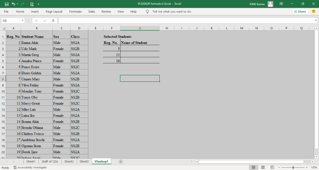
Let us illustrate with a simple example. The worksheet below displays the detail of students in SS2 in a given school. A random sample of 3 students was selected based on their Reg. Nos.: 5, 11, and 16. Use the Vlookup formula in Microsoft Excel to retrieve the names of the students.
The vlookup formula in excel is written as follow: =VLOOKUP(Reg. No., in worksheet range, column no. in the worksheet range, [exact/Approximate match])
The above explanation will result in the following: =VLOOKUP(F3,$A$2:$D$21,2,TRUE).
Notice that:
- The F3 is the cell reference of the first Reg. No. (5). If you copy the formula to the remaining cells, all the results will appear accordingly. You may decide to use the Reg, No., instead of cell reference if you are dealing with a few values. In this case, you will have =VLOOKUP(5,$A$2:$D$21,2,TRUE).
- The absolute range reference $A$2:$D$21 references the range that contains the data we are searching for. We used absolute reference style so that when we copy the formula, the range will not change. You can also convert the range to a table or name the range. If you do either, you will have something like this: =VLOOKUP(F3,Random_search,2,TRUE), where the Random_search is the name of the range. If you used a table, then, =VLOOKUP(F3,Table1,2,TRUE). Naming the range allows you to copy the formula without changing the scope of the data.
- The value “2” is the column index or column number within the range where what I am looking for can be found. Looking at the worksheet, you find out that the student’s name is in column 2, counting from the left.
- The last entry is optional. You can decide to omit it and still have the same result. TRUE stands for approximate match and is the default value. FALSE means exact match. TRUE usually selects a value close to or less than what you are searching for. But FALSE selects the exact match of what you are looking for.
The result of the vlookup formula is given below, check if your result is close to it.
What is Vlookup Formula in Excel?
The vlookup formula in Excel is one of the legacy functions that has been part of Excel since its inception. It is one of the most used functions in the history of Microsoft Excel. It is used to query data to retrieve a value based on available data input.
To use the vlookup formula, we must organize data in columns. The data is usually arranged such that the lookup value is to the left of the return value. Columns are numbered from the left to the right, indicating the column indexes, as shown below.
| Reg. No | Student Name | Sex | Class |
| 1 | Emma Akin | Male | SS2A |
| 2 | Udo Mark | Female | SS2B |
| 3 | Martin Greg | Male | SS2A |
| 4 | Amaka Prince | Female | SS2B |
| 5 | Peace Evere | Male | SS2C |
| 6 | Ebere Golden | Male | SS2A |
To retrieve a value using the vlookup function, we will provide the column index. The column index represents the column number within the data range. For example, in the above table, to retrieve sex, the column index is 3.
When using the vlookup function in Excel, the retrieved value must be to the right of the lookup value. This means that if you are looking up student names to retrieve the Reg. No. Then, the Reg. No. must appear to the right of the student’s name.
The syntax of the vlookup function in excel
The syntax of the vlookup function in excel is given by: =VLOOKUP (lookup_value, table_array, col_index_num, [range_lookup])
Where:
- lookup_value is required. It must be specified and represents the value you are looking up for, e.g. Reg. No. The secret of using the vlookup function is that the lookup value MUST be in the column index 1. That is, it must be in the first column of the range of data specified in the table_array. In our example above, notice that the Reg. No appeared in the first column (Column A) of the range $A$2:$D$21. The lookup value can be a value, a text, or a cell reference.
- table_array is required also. This represents the range or table where the vlookup function will search for the lookup_value to retrieve the value. Remember that the first column in this range must contain the lookup_value. The table_array can be a range of cells using cell reference, a named table, or a named range. The value to retrieve must be inclusive in the table_array for the vlookup function to return a value.
- col_index_num is also required. This is the column number that contains the value to be retrieved by the vlookup function. Remember that the columns should be numbered from left to the right beginning with the column that contains the lookup_value. That is, within the table_array count from the left-most (that contains the lookup_value) to the column that contains the return value.
- range_lookup is optional. This is used to tell the vlookup function to look for an approximate or exact match of the lookup_value. It is a logical value of TRUE or FALSE which can be written as 1 or 0 respectively. TRUE is the default value and searches for the closest value specified in the lookup_value column. FALSE or 0 searches for the exact value specified in the lookup_value column.
The exact and approximate match in the vlookup function
Range_lookup = TRUE
To use the approximate match (TRUE) option in the vlookup formula, always sort the first column in ascending order. If the value is not sorted, the return value might be wrong. This is because vlookup will look for the value equal to or smaller than the lookup_value specified.
If the lookup_value is smaller than the least value in the first column (lookup_value column), then the function will return #N/A.
Let us illustrate with the following example. In the worksheet below, the score of the student will determine if he/she is promoted, demoted, or not promoted. The status table is given as follow:
| Score Range | Remark |
| 0 – 50 | Demoted |
| 50 – 75 | Not Promoted |
| 75 – 100 | Promoted |
In the worksheet below, I purposely started with 50 instead of 0 to illustrate how TRUE works. The vlookup formula is given as follows: =VLOOKUP([@Score],$G$8:$H$10,2,TRUE), with the following result.
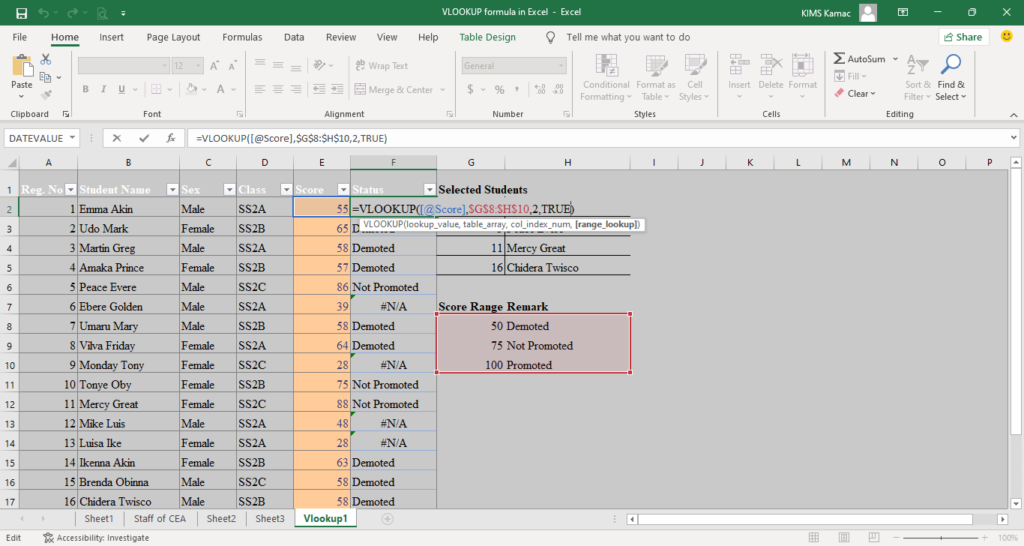
Notice that all values below 50 have the status of #N/A. This is because the lookup_value is smaller than the value looked up in the table_array. It, therefore, looks for an approximate match and returns a #N/A error if it did not see any.
Also, notice that all scores below 75 have a status of demoted. This is because TRUE in the range_lookup will return values equal to or smaller than the lookup_value.
Range_lookup = FALSE
If the exact match (FALSE) option in the vlookup formula is used, vlookup will return the exact match. If the exact lookup_value is not found in the first column (lookup_value column), then the function will return #N/A.
For example, using the above example, change the TRUE in the range_lookup to FALSE, to get the following result:
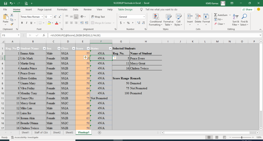
Notice that only a score of 75 returned a correct status. Others displayed #N/A. This is because there is no exact match.
Important notice
When using the vlookup formula in Excel, it is necessary to do the following:
- Always sort the first column in the table_array (column that contains the lookup_value), especially when using approximate match. Remember that approximate match is activated when the range_lookup is TRUE or 1.
- Always use absolute referencing, or a named range, or a named table when defining the table_array. This is important, especially when you want to copy the formula to other cells.
- Always store values appropriately to avoid incorrect results. Store numbers as NUMBERS, date as DATE, and text as TEXT. If you store the number as text, you will get incorrect results.
- Use wildcard characters in the vlookup function when range_lookup is FALSE and lookup_value is a text. Remember that “?” matches a single character and “*” matches a sequence of characters. This can be used, when using the exact match (FALSE) in the range_lookup and the lookup_value is a text, if necessary.
How to use Vlookup Function in Excel
As one of the most used functions in Microsoft Excel, every Excel user must understand it. We shall illustrate how to use the vlookup formula in Excel using the following examples.
Example 1: Simple use case
The worksheet represents the sales record of a given trading company. Five products were selected from the sales record: Festo biscuit, Minimie 100g, Nibit, Coca cola, and Viva 190g. The management wants to know who sold them and the selling price. Use the vlookup function in Excel to retrieve the required values.
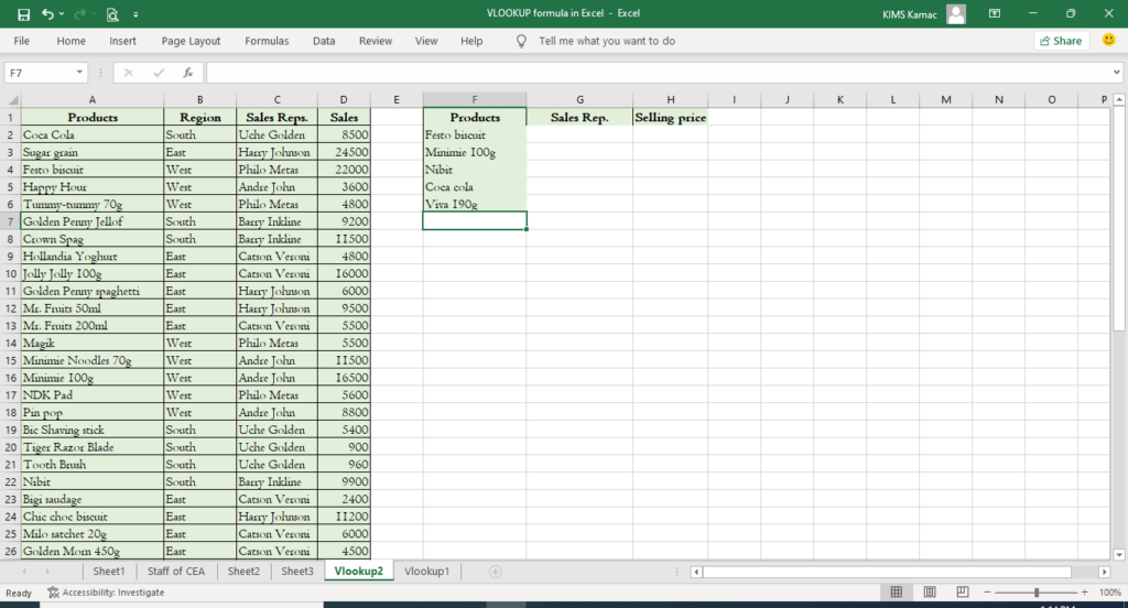
To solve this problem, we follow these steps.
- Enter the required data in a worksheet or import the data from any source.
- Create three columns within the worksheet and label them accordingly. See the example above.
- Select the entire range of cells that contain the data and name it salesdata. Ensure that the first column contains the products because this contains our lookup_value. This range is our table_array. Please, don’t include the headers, i.e. products, Region, etc in the table_array.
- Label the columns from left to right: we have 4 columns starting with Products as 1 and sales as 4. These are our col_index_num.
- On cell G2, enter the following formula =VLOOKUP(F2,salesdata,3,FALSE). Note: we are using an exact match.
- Copy the formula to the other cells below G2 using the autofill handle.
- On cell H2, enter the following formula =VLOOKUP(F2,salesdata,4,0). Note that you can use either FALSE or 0 for an exact match.
- Copy the formula to the other cells below H2 using the autofill handle.
The result is shown in the table below. Your result should look like this.
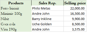
We were able to use the vlookup function to query our data table and retrieve the values shown above. This is a simple scenario.
Example 2: Using vlookup in the place of IF function.
The table below shows the results of students in a given secondary school. The grade obtained by each student is distributed using the following table.
| S/N | Score Range | Grade |
| 1 | 85 – 100 | Excellent |
| 2 | 70 – 85 | V. Good |
| 3 | 60 – 70 | Good |
| 4 | 50 – 60 | Pass |
| 5 | 0 – 50 | Fail |
The average score of each student is shown in the worksheet below. Use the vlookup function in Excel to grade each student based on their scores.
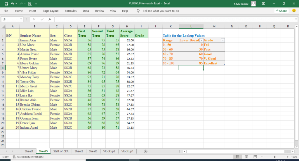
To solve this problem, we create a table for the lookup value using the range and the grades as follow:
- Create the table for the lookup values and ensure that they are in ascending order as shown above.
- Create a column within the table above which contains the lower bound of each range. This column will be the lookup_value column and the first column in the table_array. Ensure that this column is arranged in ascending order, see worksheet above.
- Highlight the lower bound column and the grades column and convert them to a table. To do this, On the Home tab, under Styles, select Format as Table. From the designs that appear select any table design.
- Name the table in 3 above gradeTbl. To do this, select a cell in the table you created. On the Table Design tab, under Properties, change the table name.
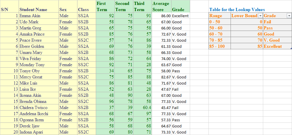
- Under grades, in column I2, enter the following formula: =VLOOKUP(H2,gradesTbl,2,TRUE). The vlookup function will search for and return values equal to or less than the lookup_value from the table_array.
- Copy the formula to other cells using the autofill handle. The results are shown in the figure below.
Conclusion
The vlookup function in Excel is very useful, though it has its weaknesses. You can use it to do different things such as retrieve a value from a data table and merge two tables.
The vlookup function can also be used with an IF function to return a different value if an error occurs. There are various use cases where you can deploy the vlookup formula in Excel. All you need is to understand how to use it.
This tutorial has helped you to build a foundational understanding of how to use the vlookup formula in Excel. If you keep practicing it in different scenarios, you will understand it more. We are open to your questions in case you face any challenges while practicing how to use the vlookup function.
There are yet other lookup functions in Excel: The Hlookup and the recently added Xlookup. The Hlookup is like the vlookup function but looks up a value in the rows rather than columns. We shall look at the Xlookup function by next week. Before you go, please, kindly share with a friend. Don’t forget to visit our previous tutorials if you have not done so.


