Conditional formatting in Excel: Uses and Applications

Conditional formatting in Excel is an important tool used for effective data analysis. It is a tool that helps you identify and critically visualize cells that have patterns and trends using colors.

Conditional formatting in Excel helps you to visualize and understand data in a worksheet without the use of charts. It is a tool that incorporates color scales, data bars, and icon set to identify variations in data patterns.

It is an interesting data analysis tool that identifies cell variations based on true data conditions. When conditions are specified, cells appearances may vary in compliance with the specified conditions.

For example, the table below displays a household’s monthly electricity consumption in 6 months. Electrical appliances that consumed lower units of electricity are highlighted with light-blue color. As the units increase, the cell color becomes dark yellow. But the appliances with greater units are highlighted with green color.

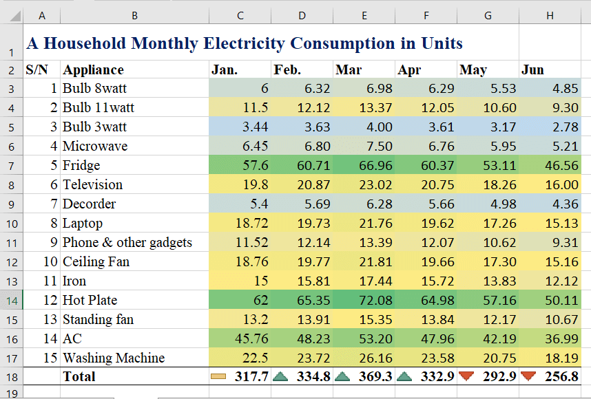
Notice that the total row, in the table above, used an icon set to show deviations from the base value. Values higher than the base value are indicated with an up-level icon. Similarly, lower values are identified with a down-level icon.

In this tutorial, we discussed what is conditional formatting in Excel and how to use them in your datasets.

Previous Excel Tutorials:

• What is Microsoft Excel: Tutorial 1
• Entering and formatting data in Excel: Tutorial 2

What is Conditional Formatting in Excel?

Conditional formatting in Excel is a tool that works like a chart. But instead of representing data in the vertical and horizontal axis, data values are represented with colors, bars, and icon sets.

In Excel, conditional formatting helps the audience to visualize data with clarity and precision without requiring further analysis.

For example, in the table above, one will easily observe the 3 electrical appliances that consume electricity units. These appliances were indicated with the green color as refrigerator, hot plate, and air conditioner.

Hence, to reduce the total electricity units consumed in a month, the household can reduce the usage of these appliances.

Thus, conditional formatting in excel is a command that helps you to identify variations in data values within a selected range. It allows you to use color scales, data bars, and icon sets to highlight data values for a clearer understanding.

Uses of conditional formatting in Excel

At what point would you use the conditional formatting in excel? Or what are the benefits or usefulness of conditional formatting in excel? From experience and usage, we can identify the following benefits of conditional formatting.

1. Conditional formatting is a mini-chart that helps you summarize data at a glance without the use of complex analysis tools. Important values can be easily identified using colors, bars, and icons.
2. It can help you detect critical issues or set trigger points within a dataset. For example, if you don’t want to spend beyond a particular amount, you can use conditional formatting to set trigger. This alert can be activated with different colors at different data values, say, at 50%, 75%, and 95%.
3. You can use it to identify unusual values. For example, monthly product sales should not be below the breakeven quantity. You can use conditional formatting to detect when such a scenario occurs.
4. It is also useful when evaluating formulas to arrive at a solution. For example, you can include a condition using a formula that evaluates to true or false.

How to copy conditional formatting in excel

You can copy the conditional formatting in a particular dataset and apply it to another dataset in Excel. You can do this using the format painter.

To copy conditional formatting, you should make sure that the two datasets are similar. You should not copy the conditional formatting of text-based data to numeric data.

Do the following when copying conditional formatting in excel.

1. Locate the conditional formatting of data you want to copy and highlight the cell or range of cells.
2. On the Home tab, under the Clipboard group, select the Format Painter.
3. Locate the data where you want to apply the copied conditional formatting on.
4. Using the format painter pointer, select the cell or range of cells you want to apply the formatting on.
5. The conditional formatting is automatically applied to the selected cells.

The quick analysis button

The quick analysis button in the Excel worksheet helps you to quickly apply formatting to your data. Whenever you highlight data in a cell or range of cells, the quick analysis button appears.

You can use this tool to apply conditional formatting instead of visiting the Home tab >> Styles group. With the quick analysis tool, you can add charts, tables, totals, and spikelines to selected data.

To use the quick analysis tool to apply formatting, do the following:

1. Select the data that you want to apply formatting to or data you want to analyze.
2. The quick analysis button appears at the lower right corner of the selected items.

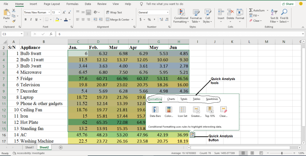
3. Click the quick analysis button to reveal the different analysis tools you can apply to the selected data.
4. To apply conditional formatting, select the Formatting tab, and choose any of the conditional formatting options.

How To Use Conditional Formatting In Excel

There are five simple ways to use conditional formatting in Excel. They include:

• Highlight cells rules
• Create top/bottom rules
• Use of data bars
• Selecting color scales, and
• Specifying icon set

Highlight cells rules

This type of conditional formatting is used to identify cells based on preset rules. There are 7 preset rules to be chosen from. They include: greater than, less than, between, equal to, the text contains, date occurs, and duplicate values.

When a cell meets the given criteria, the specified color is highlighted on such cell. To apply this type of conditional formatting, do the following:

1. Highlight the cell or range of cells you want to apply conditional formatting on.
2. On the Home tab, under Styles, select Conditional Formatting.

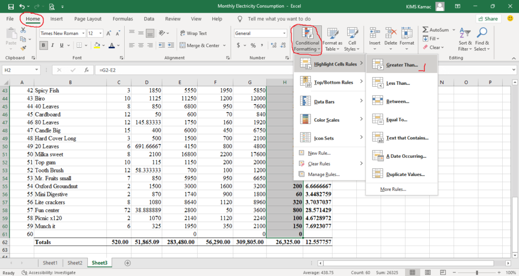
3. From the dropdown menu, point to Highlight Cells Rules and select Greater than… Note:You can select any of theoptions available depending on the rule you want to set. For example, if you are setting a less than rule, select Less than…
4. A dialog box appears.

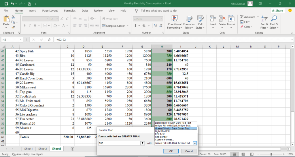
5. On the dialog box, specify the greater than value in the text box.
6. Then select the type of highlight for cells greater than the specified values in the With dropdown box. Notice the effect on the selected cells.
7. Click OK when done. The specified formatting will be automatically applied.

You can also use this method to highlight cells which has a particular text value. Also, cells that have values between two values can be identified, and cells with duplicate values.

Create top/bottom rules

This type of conditional formatting can be used to set targets and cutoff points in data. For example, in an academic section, we can set a target for top and least performing students.

Let us assume that the average student scores 55% in the overall assessment. Using the top/bottom rule, we can identify students that scored above average or those that scored below average.

To use the top/bottom rule, do the following:

1. Highlight the cell or range of cells you want to apply conditional formatting on.
2. On the Home tab, under Styles, select Conditional Formatting.
3. From the dropdown menu, point to Top/Bottom Rules and select Top 10%… Note:You can select any of theoptions available depending on the rule you want to set.
4. A dialog box appears.
5. On the dialog box, specify the top% value you want, e.g. 10 or 20, etc, in the text box.
6. Then select the type of fill for cells that meet the criteria in the With box.
7. Click OK when done. The specified formatting will be automatically applied.

You can also use this option to identify values above or below average, and top 10 or bottom 10 values.

Use of data bars

A data bar is used to compare values in selected cells or ranges. When a data bar is used, the length of the bars depicts the value in a cell. Higher values have longer bars while lower values have shorter bars.

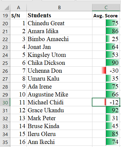
Data bars can also be used to specify negative and positive values in a range of cells. Data bars with negative values will extend leftwards, while positive values extend rightwards. However, you should configure the data bars to start from the middle of the cells.

To apply data bars conditional formatting in Excel, do the following:

1. Highlight the cell or range of cells you want to apply conditional formatting on.
2. On the Home tab, under Styles, select Conditional Formatting.
3. From the dropdown menu, point to Data bars and select any of the preset data bars.

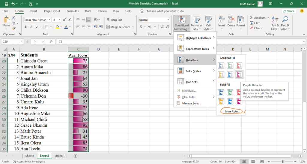
4. The specified formatting will be automatically applied to the selected cells.

You can choose between Gradient Fill and Solid Fill. You can also specify your own rules by clicking the More Rules… When you choose the More Rules button, you will be able to set up your own conditional formatting rules.

If you selected the More rules option, then do the following:

5. The New Formatting Rule dialog box will appear.

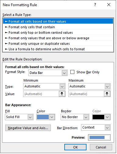
6. On the dialog box that appears, under Bar Appearance: change the Solid Fill to Gradient Fill. Choose a color of your choice. I chose a green color.
7. Select the Negative Value and Axis… button. A dialog box will appear.

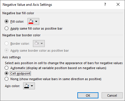
8. On the dialog box, leave the negative bar fill color as red. Change the Axis settings to Cell midpoint.
9. Click OK.
10. Click OK on the New Formatting Rule dialog box.
11. The rule will be automatically applied as shown below.

Selecting color scales

Color scales are visual guides that perform a similar function as the data bars. The difference is that color scales use color gradations and variations to interpret the difference between two values.

There are two types of color scales: two-color and three-color scales. Color scale usually compares lower and higher values by using color variations.

In a two-color scale, lower values are represented with color, e.g., blue, and the higher values with green. Values between the low and high values transform from blue to green depending on the value.

On a three-color scale, you can represent low, middle, and high values with three different colors. These colors will keep varying depending on the value of a cell with high values shading the high color.

To use the color scale conditional formatting in excel, do the following:

1. Highlight the cell or range of cells you want to apply conditional formatting on.
2. On the Home tab, under Styles, select Conditional Formatting.
3. From the dropdown menu, point to Color Scales and select any of the preset color scales.
4. The color scale will be automatically applied to the selected range.
5. If you selected the More Rules… option, then do the following:
6. The New Formatting Rule dialog box will appear.

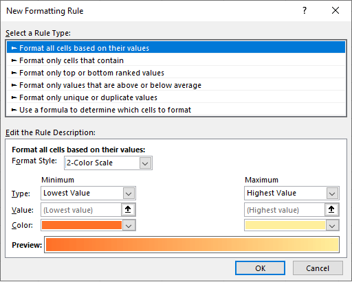
7. On the dialog box that appears, under Format Style: choose either two-color or three-color scale.
8. Choose a color for the minimum value, and the maximum value respectively.
9. Click OK when done. The rule will be automatically applied.

Specifying icon set

The icon set is used to classify values. Each category is separated by a value or range of values. There is different icon set, and you can customize your own icon set. Each of the icons in the set represents lower, middle, and upper values.

To use icon set in conditional formatting, do the following:

1. Highlight the cell or range of cells you want to apply conditional formatting on.
2. On the Home tab, under Styles, select Conditional Formatting.
3. From the dropdown menu, point to Icon Sets and select any of the preset icon sets.

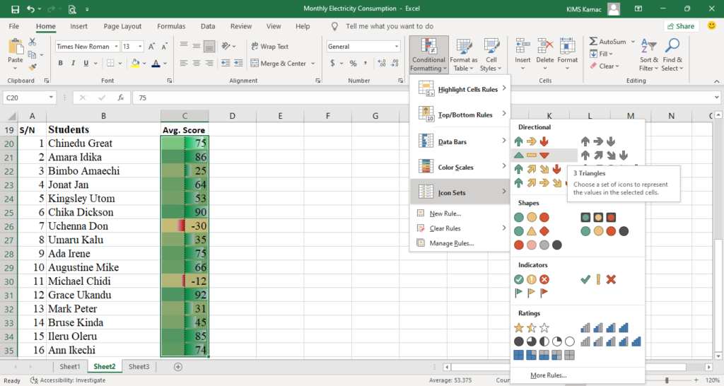
4. The selected icon set will be automatically applied to the selected range.
5. If you selected the More Rules… option, then do the following:
6. The New Formatting Rule dialog box will appear.

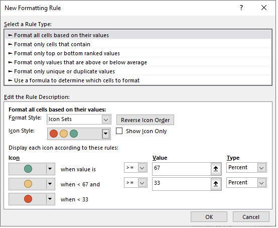
7. On the dialog box that appears, under Icon Style: choose any of the icons set from the list.
8. Under Icon, represent each icon based on the anticipated cell value or range of value. You can also change the icon if you want.
9. Click OK when done. The rule will be automatically applied.

Conditional formatting in excel formula

You can use a formula to determine how a cell or range of cells will be formatted. Conditional formatting in Excel formula requires that you specify a logical condition that must evaluate to TRUE/FALSE.

The true value is represented with 1 and the false value is represented with 0 in the function. For example, we will use a formula to highlight cells that have their margin greater than or equal to 650.

To apply conditional formatting using Excel formula, do the following:

1. Highlight the cell or range of cells you want to apply conditional formatting on.
2. On the Home tab, under Styles, select Conditional Formatting.
3. From the dropdown menu, select New Rule… The New Rule dialog box will appear.

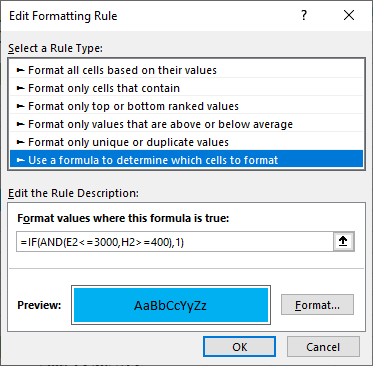
4. On the dialog box, under Select a Rule Type, select Use a formula to determine which cells to format.
5. In the text box, enter a formula that evaluates to true/false. E.g., [=ISEVEN(A2); =IF(H2>=650,1); =IF(AND(E2<=3000,H2>=400),1), etc.]
6. Select the Format… button and choose a color of your choice.
7. Click OK to return to the new rule dialog box.
8. Click OK to apply the specified rule. The rule is automatically applied.

Conditional formatting in excel based on another cell

You can also use conditional formatting to format a cell based on the value of another cell. For example, we shall use conditional formatting to select the products which cost is less than 5000, and whose margin is greater than or equal to 500.

Do the following:

1. Highlight the cell or range of cells you want to apply conditional formatting on.
2. On the Home tab, under Styles, select Conditional Formatting.
3. From the dropdown menu, select New Rule… The New Rule dialog box will appear.
4. On the dialog box, under Select a Rule Type, select Use a formula to determine which cells to format.
5. In the text box, enter the formula [=IF(AND(E2<=5000,H2>=500),1)]
6. Select the Format… button and choose a yellow color.
7. Click OK, then click OK. The cells that meet the condition will be automatically selected as shown below.

Clear Conditional Formatting in Excel

To remove conditional formatting in Excel, do the following:

1. Highlight the cell or range of cells you want to remove conditional formatting on.
2. On the Home tab, under Styles, select Conditional Formatting.
3. From the dropdown menu, point to Clear Rules…
4. From the list that appears, select either:
   • Clear Rules from Entire Sheet (clears all rules in the worksheet)
   • Clear Rules from Selected Cells (Clears all rules in the selected cells)

Conclusion

Conditional formatting in Excel is an interesting tool that helps you quickly summarize and analyze data. It is easy to apply and it visualizes data for clarity and ease of comprehension.

We discussed in this tutorial, what is conditional formatting in Excel. Here we discussed conditional formatting and its uses.

We further looked at how to use conditional formatting in Excel. Here we identified five ways of applying conditional formatting with examples.

We finally looked at how you can use a formula to apply conditional formatting. There are few things we did not cover: managing rules in conditional formatting. If you have a question regarding this, please, indicate it in the comment section. Next week we shall continue with formatting numbers and worksheets in Excel.