PivotTable in Excel is an advanced tool that allows you to organize and analyze large data set. Using pivot tables, you can extract data from a large dataset, and present the summary or analysis of such data.
PivotTables help you to easily see patterns and trends and easily make comparisons of data in a table. You can easily summarize large data using functions such as Sum, Count, Average, etc.
For example, the Pivot Table below summarized the number of students registered for the new section in a given secondary school. A total of 258 students were registered into different classes from SS1 to SS2.
Pivot Tables Explained
PivotTables are used to summarize data, especially, when the available data is large. With it, you can easily identify variations and seasonality in data. You can also view data from different perspectives with just a click using PivotTables.
For example, in the above table, we can view the total number of registered students by sex or by class.
PivotTable in Excel 1993 – 2007
Pivot table has been part of Microsoft Excel since 1993 when it was included in Microsoft Excel 5. Since then, Microsoft has improved on the functionality of the pivot table as new versions of Excel are released.
For instance, The Excel 1997 version included the pivot table wizard and the ability to create calculated fields. The Excel 2000 version added a pivot chart to graphically represent pivot table data.
In 2007, the Excel version improved how to work with PivotTables by making it a lot easier to work with. It becomes easier to interact with the fields on the pivot table workspace.
PivotTable in Excel 2010
In 2010, a new feature was added that assists users to quickly customize pivot tables with a click. Then, you can easily change pivot table summary types and calculation types from the ribbon with a click.
PivotTable in Excel 2013
In 2013, a timeline was added to pivot tables. Timelines allow you to filter records in a PivotTable by dates.
To add a timeline in Excel 2013, select the PivotTable and click on the contextual Analyze tab. Under the filter group, select insert timeline. A dialogue box appears from where you will customize your timeline.
PivotTable in Excel 2016
In 2016, the search field was included in the pivot table. This makes it easier to search for fields within the pivotable, especially, when working with many fields. It also eliminates confusion, saves time, and makes working with fields in the pivot table easier.
PivotTable in Excel has witnessed a lot of improvements since its inception. These improvements have made working with PivotTables easier and made the skill important among Excel users.
What is the use of PivotTable in Excel?
Generally, a pivot table is used to organize a large volume of data so anyone can easily understand them. The use of a pivot table depends on the volume of data and what the user wants to achieve.
Looking at the above example as a guide, we can say that the uses of PivotTables include the following:
- To summarize a large volume of data. For example, the registered students were summarized using Sex and Class. Generally, we can easily deduce the number of students that were registered, and the number in each class.
- To sort and filter data. The pivot table provides an option that assists users to sort data in ascending or descending order. You can also decide to filter data using data labels or based on categories.
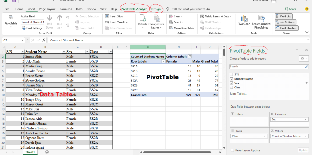
- To organize and reorganize data into groups or categories. You can organize data in columns and rows, and reorganize data in rows and columns using different fields. To achieve this, you can simply add fields to column or row labels.
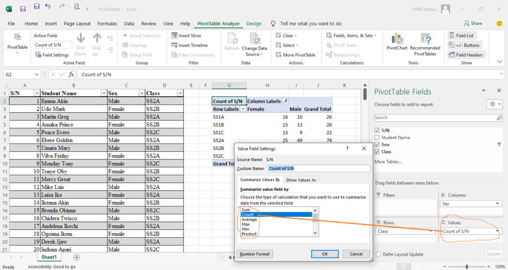
- To analyze data with the aid of functions. The summary of the data can be obtained by performing necessary calculations using preset functions. The values field allows you to select any function of your choice to summarize your data. You can use the SUM, COUNT, AVERAGE functions, etc. In our example above, we used the COUNT function to summarize our data.
- To perform data comparison. You can compare data by using a multi-dimensional table to figure out differences and trends in data units.
How to create a PivotTable in Excel 2016
To create a PivotTable in Excel, especially Excel 2016 and 2019, do the following:
- Open the worksheet that has the data you want to summarize or type the data in a worksheet. If you wish, convert the data to a table.
- Select a cell anywhere outside the data table. Though you can choose to insert the pivot table in another worksheet.
- On the Insert tab, under the Tables group, select PivotTable.
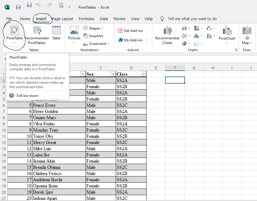
- The PivotTable dialog box appears.
- On the PivotTable dialog box, under Table/Range enter the name of the table or highlight the entire data range.
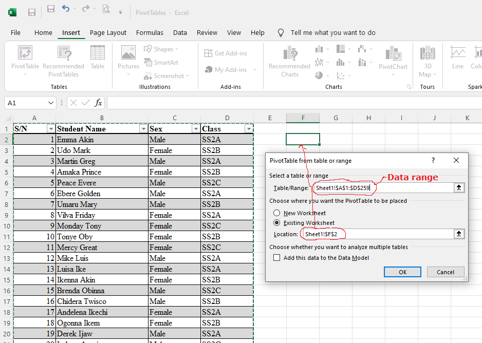
- On the dialog box, under Choose where you want the PivotTable to be placed, select Existing worksheet. Then select a cell location within the worksheet. See the image above.
- Click OK on the dialog box to display PivotTable fields and PivotTable workspace.
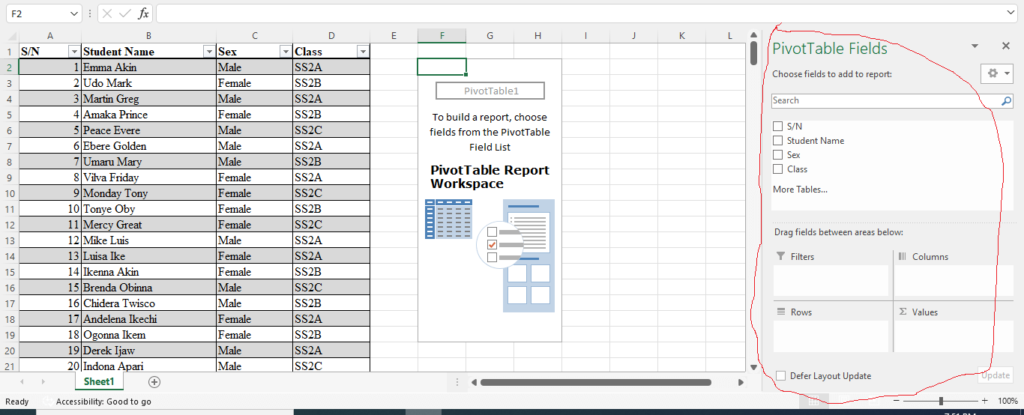
- On the PivotTable fields, select the fields you want to display. Move any of the fields to the rows or columns depending on how you want the summary.
- To filter the results, move a field to the filter area.
- To compute the summary of the data, move the summary field to the values area and choose a function. When you move a field to the values area, the COUNT or SUM function is automatically selected.
- The results of the selected fields are displayed in the PivotTable report workspace as shown below.
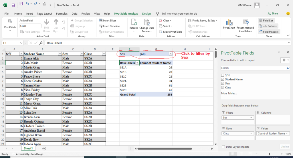
PivotTable Example
Haven understood how to create a PivotTable in Excel, let us illustrate how to use the PivotTable.
The worksheet below shows the sales record of Bluewy Inc. for September. Use the pivot table to analyze the data.
Firstly, let us create the PivotTable using the above steps. The image below displays the PivotTable Example using the Bluewy sales record.
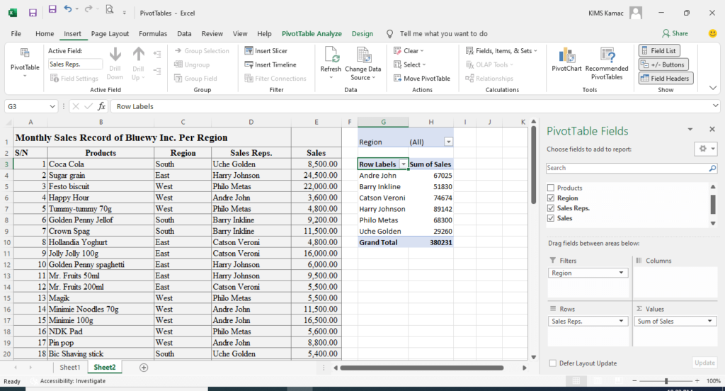
On the PivotTable, we can perform the following as discussed above. Sort data, filter data, summarize data, and compare data.
Sort data in PivotTable
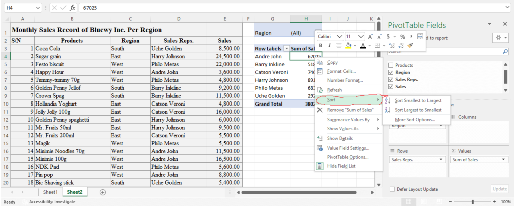
On the PivotTable report workspace, right-click a cell under Sum of Sales. And point to Sort. Select either ascending order or descending order.
You can also click the Row Labels and sort either ascending or descending order. You can also filter based on the rows categories.
Filter data in PivotTable
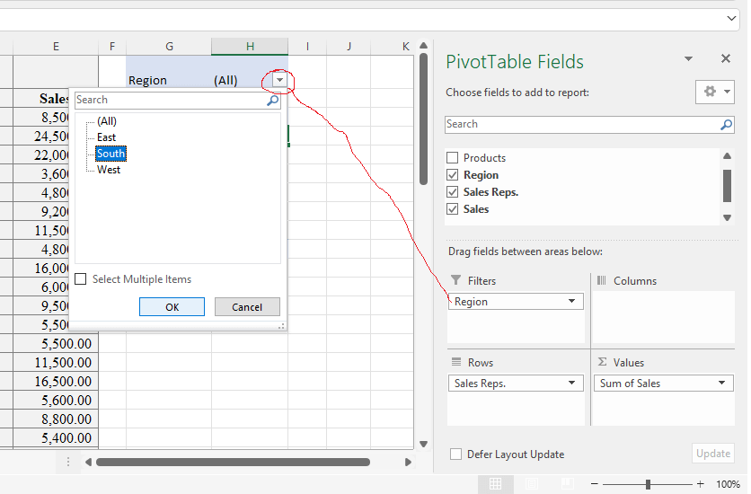
Add a field in the filter area of the pivot table field. We added a region in the filter area.
On the PivotTable report workspace, click the filter button and select any of East, South, or West and click OK.
Perform data comparison
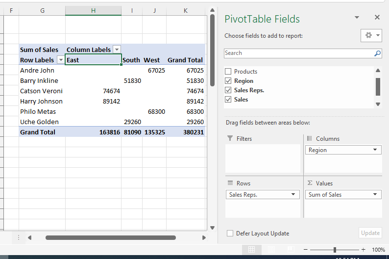
To create a multi-dimensional table and make a data comparison you will add a field in the row area and another in the column area.
In the Pivot table above, move regions to the column area and Sales reps to the row area. You have created a multi-dimensional table that will help you compare the sales in different regions and sales reps.
Conclusion
The PivotTable is a skill that is important in today’s world. This has made it necessary for students, applicants, and users of Excel to seek its knowledge.
The tutorial thus far has illustrated how to use PivotTable in Excel. It is quite simple to create a pivot table for any use you want.

