Excel, a powerful tool for data analysis and manipulation, is not immune to errors. From simple division by zero to complex formula miscalculations, errors can disrupt your work and hinder productivity. However, with the right tools and techniques, you can gracefully handle these errors and ensure the accuracy and reliability of your spreadsheets.
In this guide, we will delve into the world of Excel’s IFERROR function. This versatile tool empowers you to control how errors are displayed, providing a more user-friendly and professional experience. By the end of this tutorial, you will be able to utilize IFERROR to effectively:
- Prevent unsightly error messages: Hide distracting error values and create a cleaner worksheet.
- Provide alternative values: Display custom messages or specific values when errors occur.
- Simplify complex formulas: Combine IFERROR with other functions to create more robust and efficient calculations.
- Enhance the overall user experience: Offer a more polished and informative presentation of your data.
Other Recommended Excel Functions that Might Be of Help:
- The IF Statement in Excel: Nested and IFS Function
- How to use PivotTable in Excel 2016
- Invoice Automation with VLOOKUP Function: Excel Magic for Freelancers
No matter your experience level as an Excel user, this guide will equip you with the knowledge and skills to master error handling and enhance your spreadsheet productivity.
Let’s embark on this journey together and unlock the full potential of the IFERROR function.
What Is The IFERROR Function In Excel?
The IFERROR function in Excel is a simple yet powerful tool for handling formula errors. It allows you to replace error values with a custom message or alternative calculation, ensuring your spreadsheet remains professional and easy to understand.
What Does the IFERROR Function Do in Excel?
Errors like #DIV/0! or #N/A can disrupt your workflow and confuse users. The IFERROR function helps by preventing errors from breaking calculations, creating clean, error-free dashboards, and making data interpretation easier for non-technical users.
This valuable tool in Excel offers several key benefits:
1. Enhanced User Experience:
- Clean and Professional Worksheets: The IFERROR function helps maintain a clean and professional appearance of your spreadsheets by suppressing error messages.
- Improved Readability: Clear and concise output, free from error codes, enhances the readability of your data.
2. Robust Formula Creation:
- Error Prevention: By anticipating potential errors and providing alternative values, you can make your formulas more robust and less prone to unexpected results.
- Simplified Complex Formulas: The IFERROR function can be combined with other functions to create intricate calculations without worrying about error interruptions.
3. Data Integrity and Consistency:
- Accurate Results: By handling errors gracefully, you can ensure that your calculations are accurate and reliable.
- Consistent Output: The IFERROR function helps maintain consistency in your data, preventing inconsistencies that can lead to incorrect conclusions.
4. Efficient Problem-Solving:
- Quick Error Identification: By using IFERROR to identify errors, you can quickly pinpoint the source of the problem and take corrective action.
- Faster Troubleshooting: The function can help you streamline your troubleshooting process, saving you time and effort.
In essence, the IFERROR function is a powerful tool that empowers you to create more robust, reliable, and user-friendly Excel spreadsheets. Understanding the benefits and mastering its usage can elevate your data analysis and reporting capabilities.
Understanding The IFERROR Syntax
The basic syntax of the IFERROR function is given by:
=IFERROR(value, value_if_error)
- value: The formula or expression to evaluate.
- value_if_error: The result to return if an error occurs.
For example,
=IFERROR(A1/B1, “Invalid”)
In the above formula, if cell B1 is zero or blank, the function returns “Invalid” instead of #DIV/0!.
Common Excel Errors the Function Handles
Before diving into the IFERROR function, let’s briefly discuss some common Excel errors:
- #DIV/0!: This error occurs when you divide a number by zero.
- For example: =A1/0 returns #DIV/0!.
- #N/A: This type of error usually occurs when the requested data is not found.
- For example: =VLOOKUP(10, A1:B10, 2, FALSE) when lookup value “10” is not found in column A, the error #N/A is returned.
- #VALUE!: When an operation is performed on a wrong data type, this type of error occurs.
- For example: =”Text”/2 returns the error #VALUE!.
- #REF!: This error appears when a cell reference is invalid or deleted.
- For example: =A1/2 returns the error #REF! if cell A1 is deleted.
- #NAME?: Finally, when a function or named range is misspelled this type of error usually occurs.
- For example: =SUMA(A1:A10) instead of SUM returns #NAME?
- Similarly, =PRODUCT(Qty,Uni) instead of =PRODUCT(Qty,Unit) returns same error.
How the IFERROR Works
The IFERROR function is a simple straightforward function that works as follows:
- Checks the value argument: It evaluates the specified value or formula.
- Returns the original value: If no error is found, the original value is returned.
- Identifies errors: If an error is detected, the function proceeds to the next step.
- Returns value_if_error: If an error is found, the value_if_error argument is returned.
How To Use IFERROR Function In Excel
Now that we understand the benefits of the IFERROR function, let’s dive into the practical steps on how to use it effectively in your Excel worksheets. By following these simple steps, you can harness the power of IFERROR to create more robust and informative spreadsheets.
Basic usage
The most basic usage of the IFERROR function is to remove the display of the zero division error #DIV/0!.
Let’s say you have a formula to calculate the average of two numbers in cells A2 and B2:
=A2/B2
If B2 contains a zero, the formula will result in a #DIV/0! error. To handle this, you can use IFERROR:
=IFERROR(A2/B2, “Cannot divide by zero”)
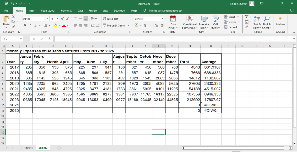
In the figure below, the average column calculated the average expenses of Deband Ventures for each year using the formula: =AVERAGE(B3:M3)
Notice that 2024 and 2025 have the #DIV/0! Error.
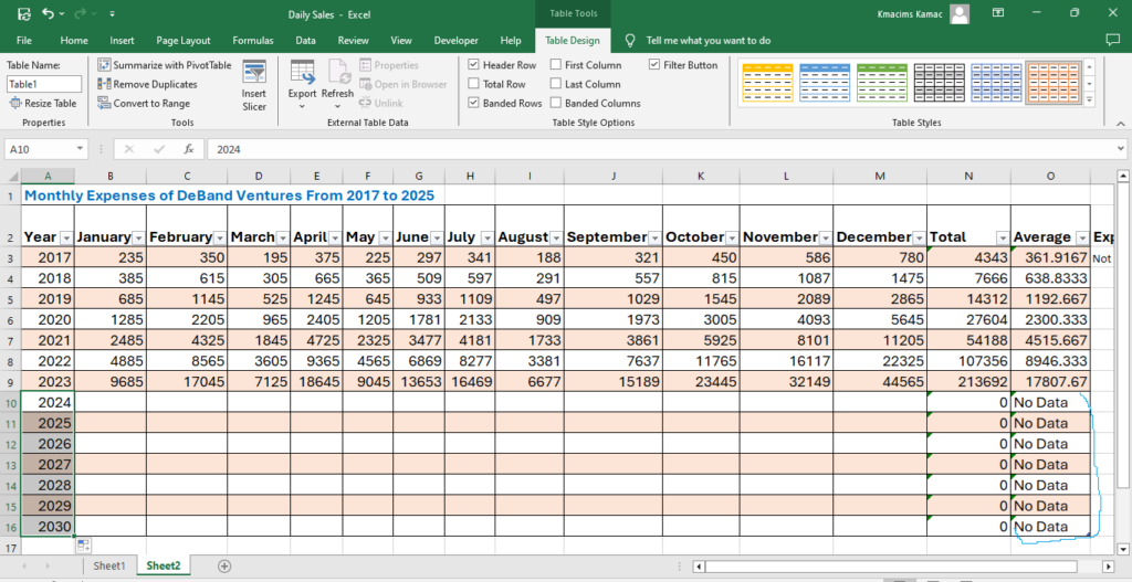
To remove this error, we can rewrite the formula to use the iFERROR function as follows,
=IFERROR(AVERAGE(B3:M3),”No Data”)
Now, instead of displaying the error, you’ll see “No Data”.
Task: Change the above formula to use the IFERROR function and view the result.
IFERROR Function In Excel Vlookup
The VLOOKUP function is often used to search for values in a table. If the lookup value is not found, it returns a #N/A error.
In the figure below, we can use Vlookup to retrieve expenses for each month of the year.
To retrieve March expenses for 2016, we use the formula:
=VLOOKUP(2016,A3:M11,4,FALSE)
Because 2016 is not in the first column, we encounter the error as shown below:

To handle this error, we can introduce the IFERROR function thus:
=IFERROR(VLOOKUP(2016,A3:M11,4,FALSE),”Not Found”)
With the IFERROR, instead of displaying the #N/A, “Not Found” will be displayed.
Creating Custom Error Messages
Displaying errors in your spreadsheet is awkward and unprofessional. You can use IFERROR to create more specific error messages to handle potential errors. This will help users understand the issue more clearly.
For example, in the above Vlookup example, you can create a specific error handler thus:
=IFERROR(VLOOKUP(2016, A3:M11, 4, FALSE), “Value not found: Please check input values”)
This will display a custom error message that will help users identify the possible source of calculation failure.
Replacing Errors with Alternate Calculations
You can also use the IFERROR to create a fallback calculation when an error occurs.
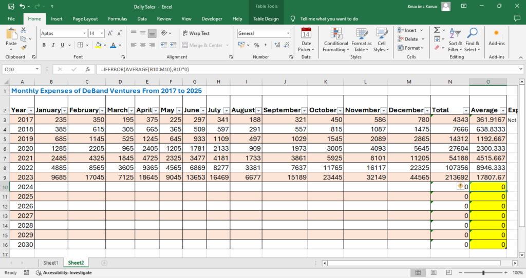
For example, while calculating the average expenses in the table below, instead of using “No Data”, we can create a fallback formula.

Hence, instead of using the formula: =IFERROR(AVERAGE(B10:M10),”No Data”)
We use this: =IFERROR(AVERAGE(B3:M3),B3*0)
The second formula will force a 0 value on rows that have no values instead of displaying the #DIV/0! Error Or “No Data” message.

Combining IFERROR with Other Functions
You can combine IFERROR with other functions to create more complex formulas, for example:
=IFERROR(SUM(B3:M3)/COUNT(B3:M3), “No data to calculate average”)
This formula calculates the average of values in the range B3:M3. If the range is empty, it displays a custom error message.
=IFERROR(PRODUCT(VLOOKUP(2019,A3:M16,5,FALSE),2),”Value Missing”)
This formula uses Vlookup to retrieve the expenses for April 2019 and multiplies the value by 2. If the value is not found, it displays the message “Value missing”.
Nested IFERROR Functions
Finally, you can nest IFERROR functions to handle multiple error scenarios in Excel.
Consider using a formula like this:
=IFERROR(IFERROR(A2/B2, “Division by zero”), “Error in calculation”)
This formula first checks for division by zero. If that’s not the issue, it checks for other potential errors and displays a generic error message.
Best Practices
- Identify Potential Errors: Before using IFERROR, analyze your formulas to identify potential error sources.
- Clear and Concise Error Messages: Provide informative error messages that help users understand the issue.
- Test Thoroughly: Test your formulas with various input values to ensure they handle errors correctly.
- Consider Data Validation: Use data validation to prevent invalid input and reduce the likelihood of errors.
By following these best practices and leveraging the power of the IFERROR function, you can create more robust and user-friendly Excel spreadsheets.
Conclusion
By mastering the IFERROR function, you can significantly enhance the reliability and user-friendliness of your Excel spreadsheets. This powerful tool empowers you to handle errors gracefully, preventing disruptions in your calculations and improving the overall presentation of your data.
Remember, the IFERROR function is just one piece of the puzzle. By combining it with other Excel functions and best practices, you can create even more sophisticated and insightful analyses.
Don’t let errors hinder your Excel journey. Start incorporating the IFERROR function into your daily workflow today! Experiment with different scenarios, explore its versatility and unlock its full potential.
By taking the initiative to learn and apply the IFERROR function, you’ll elevate your Excel skills and achieve greater efficiency and accuracy in your data analysis tasks. Before you go, do not forget to tell us your experience, questions, and suggestions. We are eagerly waiting to hear from you.


