Welcome to Part 6 of our 10-part Excel mastery series for freelancers. In this part, we will guide you through creating a sophisticated business expense tracker in Excel leveraging the powerful SUMIFS function for precise budget management, and providing a visual analysis of your expenses using sparklines.
As a business owner, effective financial management is crucial to ensure your business’s sustainability.
According to CostAnalysts, effective expense tracking helps businesses monitor their spending, identify trends, and make informed financial decisions. It can also improve cash flow and reduce taxable income (FreshBooks, September 2024).
HBS noted that proper budget management is crucial for business success. It helps allocate resources effectively, plan for future expenses, and avoid overspending.
Also, businesses that implement effective expense tracking and budget management practices often see improved financial performance and increased profitability (FreshBooks, September 2024).
In light of the above, there are different business expense trackers you can use to manage your business expenses. But these expense-tracking apps, in addition to cost, may be overwhelming to use.
As a small business, one of the most powerful tools in your arsenal is Microsoft Excel, specifically, the SUMIFS function.
Here, I’ll show you how to create a powerful business income and expense tracker for effective budget management.
Setup The Business Expense Tracker Workbook
Are you ready to take control of your finances and elevate your business to new heights? Welcome to the exciting beginning of your journey to financial mastery!
In this section, we’ll set up your business expense tracker workbook, transforming your chaotic expenses into a clear, organized, and powerful tool for success.
Imagine having a crystal-clear view of your budget, knowing exactly where every dollar goes, and making informed decisions like a seasoned CFO. This is your chance to take charge, streamline your finances, and pave the way for growth and success.
We’ll guide you step-by-step through creating essential columns, inputting sample data, and structuring your tracker to perfection. By the end of this section, you’ll have a robust foundation ready for detailed expense categorization and analysis.
Let’s dive in and build your customized Excel budget tracker. The future of your business starts now!
Keep reading and let’s make your financial dreams a reality!
Workbook organization
We’ll organize our business expense tracker in 4 worksheets, namely, Information, Expenses, Income, and Dashboard. Let’s get started!
Step 1: Create the Workbook
- Open Microsoft Excel:
- Save the workbook with a descriptive name like “Business Income and Expense Tracker”.
Step 2: Setup the Worksheets
- Rename Default Worksheet:
- By default, Excel opens with one worksheet named “Sheet1”. Right-click on it and select “Rename” to change it to “Instructions”.
- Add New Worksheets:
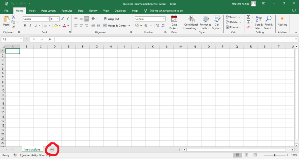
- Click on the “+” icon next to the “Instructions” sheet to add three more sheets.
- Rename them to “Expenses”, “Income”, and “Dashboard” respectively.
Structure the Worksheets
Step 1: Instructions Sheet
- Click on the “Instructions” tab.
- In cell A1, add a title like “Business Expense Tracker: Instructions”.
- Below the title, provide a brief description and step-by-step instructions on how to use the business income and expense tracker.
- Remove the gridlines: On the View tab, under Show, deselect “Gridlines”.
Step 2: Expenses Sheet
- Set Up Columns for Expense headers:
- Click on the “Expenses” sheet.
- Set up the following columns in row 1: A: Date, B: Description, C: Category, D: Budgeted Amount, E: Actual Amount
- Customize the expense headers.
- Enter Data:
- Enter data in the expense’s worksheet, beginning with your budgeted amount.
- If you do not have data, use hypothetical data for testing. You can copy the sample data provided below.
- Convert the Range into a Table:
- Select the entire data, Go to Insert > Table
- Name your table “ExpenseData”
Step 3: Income Sheet
- Set Up Columns for Income headers:
- Click on the “Income” sheet.
- Set up the following columns in row 1: A: Date, B: Description, C: Category, D: Budgeted Amount, E: Actual Amount
- Customize the income headers.
- Enter Data:
- Enter data in the income worksheet, beginning with your budgeted amount.
- If you do not have data, use hypothetical data for testing. You can copy the sample data provided below.
- Convert the Range into a Table:
- Select the entire data, Go to Insert > Table
- Name your table “IncomeData”
Step 4: Dashboard Sheet
- Design Income Layout:
- Click on the “Dashboard” sheet.
- In cell A1 type “Income Summary” and format it appropriately.
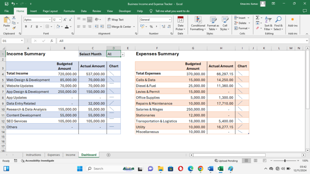
- In cell A4 enter Total Income; then in B3 Enter Budgeted Amount, and in C3 enter Actual Amount.
- In cells A5 to A13 type the following income categories
- Web Design & Development
- Website Updates
- App Design & Development
- App Updates
- Data Entry Related
- Research & Data Analysis
- Content Development
- SEO Services
- Others
- Highlight the range A3:C14 and convert it to a table. Name the table “IncomeSummary”
- Design Expense Layout:
- Click on the “Dashboard” sheet.
- In cell F1 type “Expenses Summary” and format it appropriately.
- In cell F4 enter Total Expenses; then in G3 Enter Budgeted Amount, and in H3 enter Actual Amount.
- In cells F5 to F14 type the following expense categories
- Calls & Data
- Diesel & Fuel
- Levies & Permit
- Office Supplies
- Repairs & Maintenance
- Salaries & Wages
- Stationaries
- Transportation & Logistics
- Utility
- Miscellaneous
- Highlight the range F3:C14 and convert it to a table. Name the table “ExpensesSummary”
- Insert Sparklines:
- Select cells $D4:$D14. On the Insert tab, under Sparklines, select “Line”.
- On the dialog box that appears, in the Data Range box, enter B4:C14, and click OK.

- Repeat the above steps for the cell ranges: Data Range – $G4:$H14; and Location Range – $I4:$I14.
Note: You can edit the categories to suit your business type. Use cell references according to your data location. The sparkline has two points, and it tells you at a glance, the slope of your budget vs the actual amount. An upward slope shows an increase, while a downward slope shows a decrease.
By following these steps, you’ll have a well-organized workbook with separate worksheets for instructions, expenses, and income, and a dashboard for visualizing your financial data. This structure will help you effectively track and manage your business finances.
Validate Categories in Your Data Worksheets
Use data validation to add a dropdown list for your income and expense categories. This will help you maintain data integrity.
- Select the Income sheet.
- Click on cell C2, first cell under categories.
- Go to Data > Data Validation.
- In the dialog box, under “Allow”, select List.
- In the Source box, enter the income categories range listed in the Dashboard sheet: range =Dashboard!$A$5:$A$14, and click OK.
- Select the Expenses sheet.
- Repeat steps 2 to 4.
- In the Source box, enter the Expenses categories range listed in the Dashboard sheet: range =Dashboard!$F$5:$F$14, and click OK.
Create a Month Filter
Use the month filter to summarize data by month of the year.
- Go to Dashboard sheet, in cell C1, type “Select Month”.
- Select cell D1, go to Data > Data Validation, and select List in the dialog box.
- In the Source box enter: All, Jan, Feb, Mar, Apr, May, Jun, Jul, Aug, Sep, Oct, Nov, Dec, and click OK.
- Change the formulas for total income: budgeted and actual to the following:
- Total budgeted amount =SUM(B5:B14)
- Total actual amount =SUM(C5:C14)
- Go to the Income sheet, add a column called Months immediately after Actual Amount.
- Do same in the Expense sheet.
- In both sheets and in months column, enter the formula: =MONTH([Date]). This will retrieve months from the date column.
- Change the formulas for total expense: budgeted and actual to the following:
- Total budgeted amount =SUM(G5:G14)
- Total actual amount =SUM(H5:H14)
Create a Year Filter
It’s your turn to create a date filter following the above steps. Create this and use the comment box to let me know how it went. Ask questions, and report your frustrations.
With the above, you can select the correct category for each of your income and expenses listed in your data sheets.
If you have not entered your data, you can start entering your data in both worksheets. Below is our sample data for income and expenses worksheets respectively.
Income data
| Date | Description | Category | Budgeted Amount | Actual Amount |
| 01/10/2024 | TechPoint Website | Web Design & Development | 85,000.00 | |
| 01/10/2024 | Site updates for 7 clients | Website Updates | 70,000.00 | |
| 01/10/2024 | Takeoff and completion of Glacials data | Research & Data Analysis | 155,000.00 | |
| 01/10/2024 | Financial posts mag job | Content Development | 55,000.00 | |
| 01/10/2024 | Technical & Onpage SEO for clients | SEO Services | 105,000.00 | |
| 01/10/2024 | Julian & Acktan AppPoint | App Design & Development | 250,000.00 | |
| 05/10/2024 | TechPoint paid | Web Design & Development | 70,000.00 | |
| 07/10/2024 | Klickfast Inc. paid an upfront conversion | Data Entry Related | 32,000.00 | |
| 07/10/2024 | Uclinal Inc updates | Website Updates | 10,000.00 | |
| 08/10/2024 | Neolite, Blockp, Glick, & DocTokit | Website Updates | 40,000.00 | |
| 10/10/2024 | Applemart & Flickbase | Website Updates | 20,000.00 | |
| 10/10/2024 | Financial posts mag job | Content Development | 55,000.00 | |
| 10/10/2024 | Julian & Acktan AppPoint | App Design & Development | 150,000.00 | |
| 10/10/2024 | BasePoint & JunFun Flight for SEO | SEO Services | 70,000.00 | |
| 15/10/2024 | Glacials data | Research & Data Analysis | 55,000.00 | |
| 20/10/2024 | Vinel water | SEO Services | 35,000.00 | |
Expenses Data
| Date | Description | Category | Budgeted Amount | Actual Amount |
| 01/10/2024 | Purchase of data | Calls & Data | 15,000.00 | |
| 01/10/2024 | Fuel and gas | Diesel & Fuel | 25,000.00 | |
| 01/10/2024 | Transport and lodging | Transportation & Logistics | 18,000.00 | |
| 01/10/2024 | Printing materials | Stationaries | 12,000.00 | |
| 01/10/2024 | Replacement for office equipment | Office Supplies | 5,000.00 | |
| 01/10/2024 | Payment for water and electricity bills | Utility | 10,000.00 | |
| 01/10/2024 | Repairs of systems | Repairs & Maintenance | 10,000.00 | |
| 01/10/2024 | Vat remittance | Levies & Permit | 15,000.00 | |
| 01/10/2024 | Payment of salaries and wages | Salaries & Wages | 250,000.00 | |
| 01/10/2024 | Other things not listed | Miscellaneous | 10,000.00 | |
| 01/10/2024 | Purchase of data for one month | Calls & Data | 7,000.00 | |
| 02/10/2024 | transport to buy stationeris | Transportation & Logistics | 550.00 | |
| 02/10/2024 | Payment for water bill | Utility | 3,780.00 | |
| 05/10/2024 | payment for electricity | Utility | 12,497.15 | |
| 05/10/2024 | Purchase of fuel | Diesel & Fuel | 11,360.00 | |
| 09/10/2024 | Repair of outside light | Repairs & Maintenance | 3,210.00 | |
| 10/10/2024 | Transport for meeting with Slacsport | Transportation & Logistics | 3,650.00 | |
| 15/10/2024 | Purchase of call cards | Calls & Data | 7,250.00 | |
| 17/10/2024 | Vat remittance for September | Levies & Permit | 11,360.25 | |
| 20/10/2024 | Transport for Mr. Slot | Transportation & Logistics | 1,200.00 | |
| 20/10/2024 | Office pins and battery | Office Supplies | 1,300.00 | |
| 20/10/2024 | Balance for fixing of Account’s furniture | Repairs & Maintenance | 14,500.00 | |
Using the SUMIFS Function for Budget Management
Understanding SUMIFS
The SUMIFS function is a powerful tool that allows you to sum values based on multiple criteria.
The SUMIFS function can handle up to 127 range/criteria pairs. This means you can categorize your income and expenses based on multiple criteria, such as date, category, actual, and budget amount.
The syntax is as follow: =SUMIFS(sum_range, criteria_range1, criteria1, [criteria_range2, criteria2], …)
Learn how to use the SUMIFS function with this resource: How to Use the SUMIF and SUMIFS in Excel
Applying SUMIFS to our Dashboard
Step 1: Calculate total Income and Expenses
- Open the Dashboard sheet.
- Enter the following formula to calculate the total budgeted income/ expense and actual income/expense amount each.
- Total budgeted income: In cell B4, enter: =SUM(IncomeData[Budgeted Amount])
- Total budget expense: In cell G4, enter: =SUM(ExpenseData[Budgeted Amount])
- Total actual income: In cell D4, enter: =SUM(IncomeData[Actual Amount])
- Total actual expense: In cell H4, enter:
Step 2: Apply SUMIFS to Income Summary
- Open the Dashboard sheet.
- Enter the following formula to calculate total budgeted income for each summary category:
- In cell B5, enter the formula:
- =IF($D$1=”All”,SUMIFS(IncomeData[Budgeted Amount],IncomeData[Category],”Web Design & Development”),IF($D$1=”Jan”,SUMIFS(IncomeData[Budgeted Amount],IncomeData[Months],1,IncomeData[Category],”Web Design & Development”),IF($D$1=”Feb”,SUMIFS(IncomeData[Budgeted Amount],IncomeData[Months],2,IncomeData[Category],”Web Design & Development”),IF($D$1=”Mar”,SUMIFS(IncomeData[Budgeted Amount],IncomeData[Months],3,IncomeData[Category],”Web Design & Development”),IF($D$1=”Apr”,SUMIFS(IncomeData[Budgeted Amount],IncomeData[Months],4,IncomeData[Category],”Web Design & Development”),IF($D$1=”May”,SUMIFS(IncomeData[Budgeted Amount],IncomeData[Months],5,IncomeData[Category],”Web Design & Development”),IF($D$1=”Jun”,SUMIFS(IncomeData[Budgeted Amount],IncomeData[Months],6,IncomeData[Category],”Web Design & Development”),IF($D$1=”Jul”,SUMIFS(IncomeData[Budgeted Amount],IncomeData[Months],7,IncomeData[Category],”Web Design & Development”),IF($D$1=”Aug”,SUMIFS(IncomeData[Budgeted Amount],IncomeData[Months],8,IncomeData[Category],”Web Design & Development”),IF($D$1=”Sep”,SUMIFS(IncomeData[Budgeted Amount],IncomeData[Months],9,IncomeData[Category],”Web Design & Development”),IF($D$1=”Oct”,SUMIFS(IncomeData[Budgeted Amount],IncomeData[Months],10,IncomeData[Category],”Web Design & Development”),IF($D$1=”Nov”,SUMIFS(IncomeData[Budgeted Amount],IncomeData[Months],11,IncomeData[Category],”Web Design & Development”),IF($D$1=”Dec”,SUMIFS(IncomeData[Budgeted Amount],IncomeData[Months],12,IncomeData[Category],”Web Design & Development”),)))))))))))))
- Copy the formula to other rows, but change the category to the correct category.
- Pro TIP: Use Find and Replace command to easily replace each category in each cell.
- Calculate the actual income amount:
- Copy the corresponding formula in the budgeted amount column and change the SUM RANGE from IncomeData[Budgeted Amount] to IncomeData[Actual Amount]
Step 3: Apply SUMIFS to Expense Summary
- Enter formula to calculate the budgeted expense amount as follow:
- Copy the formula in cell B5, and paste it in cell G5
- Use find and replace command to replace the Sum range to (ExpenseData[Budgeted Amount])
- Change the category to “Calls & Data”
- Copy the formula to other cells and change their respective categories.
- Enter formula to calculate actual expense amount:
- Copy corresponding formula from budgeted column to actual amount column.
- Use find and replace command to replace the Sum range from (ExpenseData[Budgeted Amount]) to (ExpenseData[Actual Amount])
- Do it for each of the cells in the actual amount column
With all the formulas in place, you can now test your business income and expense tracker to see how the dashboard summarizes your data. Edit your data by adding different months, and use the month filter to view results.
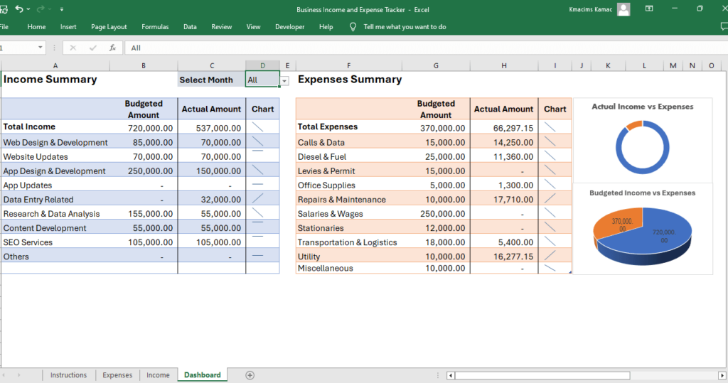
If you followed through to this point, your dashboard should look like this:

Conclusion
Congratulations! You’ve now set up a dynamic business expense tracker in Excel using the SUMIFS function for complex budget management and sparklines for visual analysis.
By mastering the SUMIFS function and incorporating sparklines, you can create a dynamic and informative budget vs. actual expense tracker.
This powerful tool will help you make data-driven decisions and ensure financial health for your business.

This tutorial is designed to help freelancers and service-based businesses manage their budgets like a pro, fostering trust and authority with detailed steps and interactive elements.
Stay tuned for more advanced Excel techniques in our next session.


