As a freelancer, managing multiple projects simultaneously can be overwhelming. One effective way to stay on top of your tasks and deadlines is using Gantt charts.
Gantt charts have revolutionized project management since their introduction by Henry Gantt in the 1910s. Today, project managers use dynamic Gantt charts for schedule visualization, keep track of and compare planned and actual timelines, and make sure that the latter is realistic and achievable.
Gantt charts are powerful visual tools for planning, scheduling, and tracking project timelines. By providing a clear overview of tasks, dependencies, and deadlines, they help project managers and teams stay organized and on track.
In this tutorial, we’ll delve into the art of creating dynamic Gantt charts in Excel, and we’ll show you how to create professional-grade charts without expensive software.
Why Gantt Charts Matter
- Clear Visual Representation: Gantt charts offer a straightforward visual representation of project timelines, making it easy to understand the project’s scope and progress.
- Task Dependency Identification: They help identify task dependencies, ensuring that tasks are completed in the correct order.
- Resource Allocation Optimization: Gantt charts aid in optimizing resource allocation by visualizing resource utilization over time.
- Risk Management: By highlighting potential bottlenecks and critical paths, Gantt charts assist in proactive risk management.
- Enhanced Communication: They facilitate effective communication between team members and stakeholders by providing a shared understanding of the project timeline.
Step-by-Step Guide to Creating a Dynamic Gantt Chart
Gantt charts are powerful tools for project management, providing a visual representation of project tasks, timelines, and dependencies.
While Excel doesn’t offer a built-in Gantt chart feature, its versatile capabilities allow you to create and customize dynamic Gantt charts.
In this section, we’ll walk you through building a dynamic Gantt chart in Excel, from setting up your spreadsheet to adding interactive elements that enhance project tracking and management.
Before we proceed these are the basic things you should have: Excel 2016 or newer version, a basic understanding of Excel formulas, and sample project data (provided below).
Step 1: Create Your Data Structure
- Open a new Excel workbook and create your data structure. You can copy and paste the sample data in the table below.
| Project Tasks | Start Date | Duration | % Complete | Dependencies |
| Planning and Strategy | 04/11/2024 | |||
| Define website goals and target audience | 04/11/2024 | 1 | ||
| Select a domain name and hosting | 05/11/2024 | |||
| Outline the website structure and content plan | 05/11/2024 | 1 | ||
| Installation and Setup | 06/11/2024 | |||
| Purchase a domain name and web hosting | 06/11/2024 | A11 | ||
| Install WordPress on your hosting account | 06/11/2024 | 1 | A14 | |
| Choose a theme (free or premium) | 07/11/2024 | 1 | A15 | |
| Design and Layout | 08/11/2024 | |||
| Customize the theme to match your brand | 08/11/2024 | 3 | A16 | |
| Create and organize pages and posts | 11/11/2024 | 2 | A15 | |
| Plugin Integration and Configuration | 13/11/2024 | |||
| Select and install essential plugins | 13/11/2024 | 1 | A15 | |
| Configure plugins | 14/11/2024 | 3 | A21 | |
| Content Creation | 17/11/2024 | |||
| Write and format content for pages and posts | 17/11/2024 | 7 | A19 | |
| Add images, videos, and other media | 24/11/2024 | |||
| Optimize content for SEO | 24/11/2024 | 2 | A24 | |
| Testing and Optimization | 26/11/2024 | |||
| Test website functionality across devices | 26/11/2024 | 2 | ||
| Optimize website speed and performance | 28/11/2024 | 2 | ||
| Ensure all links and forms work correctly | 30/11/2024 | 2 | ||
| Launch and Promotion | 02/12/2024 | |||
| Publish the website | 02/12/2024 | 1 | A30 | |
| Promote the website | 03/12/2024 | 2 |
Step 2: Set Up Named Ranges
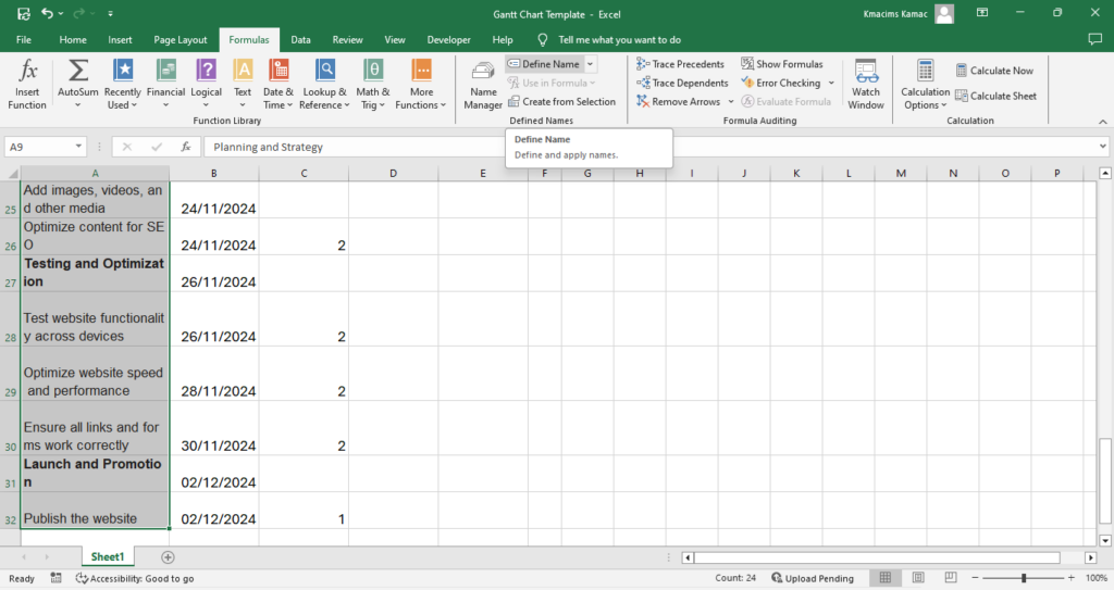
Select different data ranges in succession and define a name for each range. Named ranges make your Gantt chart dynamic and easier to maintain.
- Select your project task range: A9:A33
- On the Formulas tab, under Defined Names group, select Define Name.
- In the dialog box that appears, enter a name (e.g. Tasks) in the Name box, leave Scope as Workbook, and click OK.

- Repeat the above steps for the following named ranged:
- StartDates (B9:B33)
- Duration (C9:C33)
Step 3: Create the Timeline Header
- Determine the project start date, e.g. [Cell B9 in our example]
- Determine the project end date, e.g. [Cell B34 in our example]
- Enter the following formula in the cell your project timeline will begin, e.g. [G8 in our example]
- In G8 enter the formula [=B9]
- In H8 enter the formula [=IF(G$8 < $B$34, G$8 + 1,”End”)
- Select H8 and drag the autofill handle rightwards to fill the date row until “End” appears.
- Format the date rows to display day and months only as follows:
- Select the entire date range
- Press CTRL + 1 on the keyboard
- On the dialog that appears, under Number tab, select Custom
- Locate “dd-mmm” under custom, or edit any similar entry if you can’t find the exact entry. Click OK when done.

We have successfully generated dates across your timeline.
Step 4: Implement the REPT Function
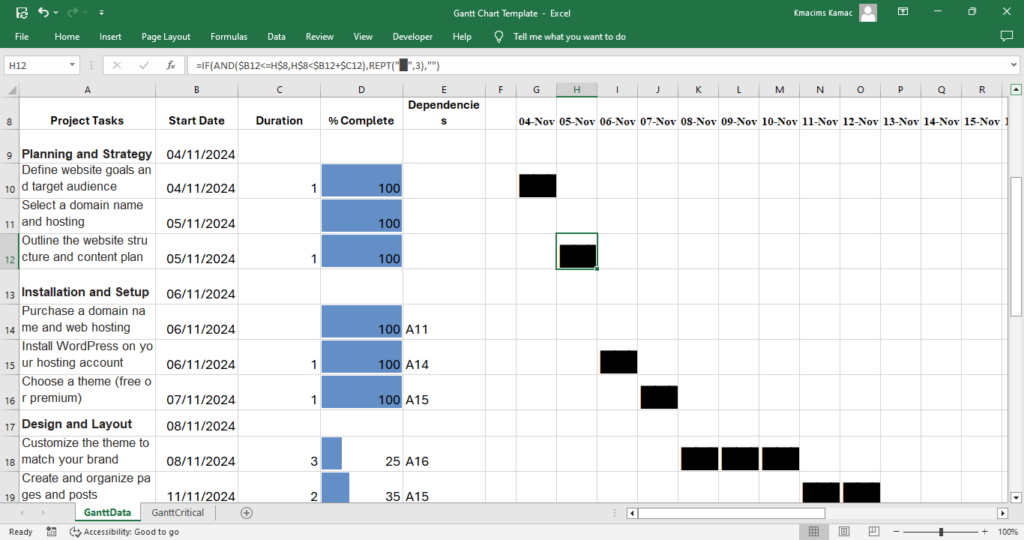
- In the first project task, under the first project timeline, enter the following formula: [=IF(AND(StartDate<=HeaderDate, HeaderDate<StartDate+Duration), REPT(“█”,1), ” “)]
- Using our example, the formula is =IF(AND($B10<=G$8,G$8<$B10+$C10),REPT(“█”,1),””)
- To get the character block “▋” hold the ALT key and press 219 on the Numeric keypad. Or insert the same from symbols.
- Copy the formula across the project timeline and tasks (use the autofill to fill rightwards and downwards).
Your Gantt chart should be similar to this:

Advanced Features
Defining the Project’s Critical Path
Here we’ll create a critical path for our project using the already-defined dependencies.
- Create a worksheet named “GanttCritical” or whatever.
- Copy and paste the basic data in the worksheet.
- Add columns for the following: Calculated Start Date, End Date, and Critical Path.
TIP: The Calculated Start Date for a task is either its given Start Date or, if it has dependencies, the day after the End Date of its dependent task.
For our example, use the formula: =IF(Dependencies=””, Start Date, End Date_of_Dependency + 1)
For our example, use the formula: =IF(E14=””,B14,G13+1). But be mindful of the dependencies.
- Calculate the project End Date using the formula: =Calculated Start Date + Duration
- The critical task is defined as a task that has dependencies and if delayed it would delay the entire project. This can be simplified by marking all tasks with dependencies as critical. Use the formula: =IF(Dependencies<>””, “Yes”, “No”)
With the above in place, we have the following refined table:
| Project Tasks | Start Date | Duration | % Complete | Dependencies | Calculated Start Date | End Date | Critical Path |
| Planning and Strategy | 04/11/2024 | ||||||
| Define website goals and target audience | 04/11/2024 | 1 | 100 | 04/11/2024 | 05/11/2024 | No | |
| Select a domain name and hosting | 05/11/2024 | 100 | 05/11/2024 | 05/11/2024 | No | ||
| Outline the website structure and content plan | 05/11/2024 | 1 | 100 | 05/11/2024 | 06/11/2024 | No | |
| Installation and Setup | 06/11/2024 | 06/11/2024 | 06/11/2024 | No | |||
| Purchase a domain name and web hosting | 06/11/2024 | 100 | A11 | 07/11/2024 | 07/11/2024 | Yes | |
| Install WordPress on your hosting account | 06/11/2024 | 1 | 100 | A13 | 08/11/2024 | 09/11/2024 | Yes |
| Choose a theme (free or premium) | 07/11/2024 | 1 | 100 | A14 | 10/11/2024 | 11/11/2024 | Yes |
| Design and Layout | 08/11/2024 | No | |||||
| Customize the theme to match your brand | 08/11/2024 | 3 | 25 | A15 | 12/11/2024 | 15/11/2024 | Yes |
| Create and organize pages and posts | 11/11/2024 | 2 | 35 | A15 | 12/11/2024 | 14/11/2024 | Yes |
| Plugin Integration and Configuration | 13/11/2024 | No | |||||
| Select and install essential plugins | 13/11/2024 | 1 | 75 | A15 | 12/11/2024 | 13/11/2024 | Yes |
| Configure plugins | 14/11/2024 | 3 | 25 | A20 | 14/11/2024 | 17/11/2024 | Yes |
| Content Creation | 17/11/2024 | No | |||||
| Write and format content for pages and posts | 17/11/2024 | 7 | 5 | A18 | 15/11/2024 | 22/11/2024 | Yes |
| Add images, videos, and other media | 24/11/2024 | 15 | 24/11/2024 | 24/11/2024 | No | ||
| Optimize content for SEO | 24/11/2024 | 2 | 0 | A23 | 23/11/2024 | 25/11/2024 | Yes |
| Testing and Optimization | 26/11/2024 | No | |||||
| Test website functionality across devices | 26/11/2024 | 2 | 10 | 26/11/2024 | 28/11/2024 | No | |
| Optimize website speed and performance | 28/11/2024 | 2 | 35 | 28/11/2024 | 30/11/2024 | No | |
| Ensure all links and forms work correctly | 30/11/2024 | 2 | 5 | 30/11/2024 | 02/12/2024 | No | |
| Launch and Promotion | 02/12/2024 | No | |||||
| Publish the website | 02/12/2024 | 1 | A29 | 03/12/2024 | 04/12/2024 | Yes | |
| Promote the website | 03/12/2024 | 2 | 03/12/2024 | 05/12/2024 | No | ||
| Completion Date | 05/12/2024 | 05/12/2024 | 05/12/2024 | No |
Create a Dynamic Gantt Chart Using Conditional Formatting
- Create the date header columns, that is the project timeline using the procedure used above. For example,
- Determine the project start date, enter the date in the first header date
- Use the manual method to add more dates column by column till the end date is reached.
- Or use the formula: =IF(ProjectStartTime < ProjectEndDate, PreviousDate + 1
- If you choose the formula, copy the formula to other columns till you reach the project end date.
- Add conditional formatting to create your chart
- Highlight the area where your Gantt chart will be visualized (e.g., J7:AQ33 if you working with our data).
- Go to the Home tab, click on Conditional Formatting > New Rule > Use a formula to determine which cells to format.
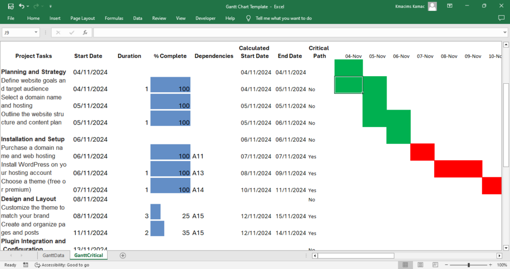
- Use the following formula to highlight the duration of each task: =AND($F8<=J$7,$G8>=J$7). This is interpreted as: J$7 is the date on the Gantt chart header (Project Timeline), $F8 is the Calculated Start Date, and $G8 is the End Date.
- Click the Format button, and apply a color of your choice. Here we used “GREEN”.
- Click OK twice to add the formatting.
- Add conditional formatting to create the critical path chart
- With your highlighted range in place, open the Conditional Formatting window > New Rule
- Add the following Formula: =AND($F8<=J$7,$G8>=J$7,$H8=”Yes”)
- Click Format and choose a color of choice, e.g. “RED”.
If you followed all the instructions, your chart should look like this:

Conclusion
Creating a dynamic Gantt chart in Excel can significantly enhance your project management capabilities by providing clear visual representations of task timelines and dependencies. Through this process, we’ve covered essential steps such as setting up your data table, calculating dependencies, and visualizing the critical path using conditional formatting.
These tools empower you to efficiently track project progress, identify potential bottlenecks, and ensure timely completion of tasks.
By leveraging the power of Gantt charts and integrating them into your project management workflow, you’re better equipped to handle the complexities of project schedules and enhance overall productivity.
As you continue to refine your skills and adapt these techniques, you’ll find even more ways to optimize your projects for success.
Ready to elevate your project management game? Start implementing Gantt charts in your Excel projects today and witness the transformation in how you visualize and manage tasks.
Share your newfound knowledge with your team and encourage them to embrace these powerful tools. Together, you’ll achieve greater efficiency and drive your projects to success.
Download a copy of the Gantt Chart template for free, and share what you learned in the comment box below.


