The SUMIF and SUMIFS in Excel are predefined functions that calculate totals based on specified criteria. You can either function to manipulate data when there are conditions associated with your data.
For example, you may want to know the total scores of female students in a class. To evaluate the total based on the condition (male students), you will employ the SUMIF function. If there is more than one criterion, you employ the SUMIFS function.
The SUMIF function is a legacy function that has been part of previous versions of MS Excel. But the SUMIFS function was introduced in MS Excel 2007 and has been useful in evaluating multiple criteria since then.
Whereas the SUMIF function accepts one criterion, the SUMIFS function accepts multiple criteria.
In this tutorial, you will learn how to use the SUMIF and SUMIFS in Excel.
The SUMIF in Excel
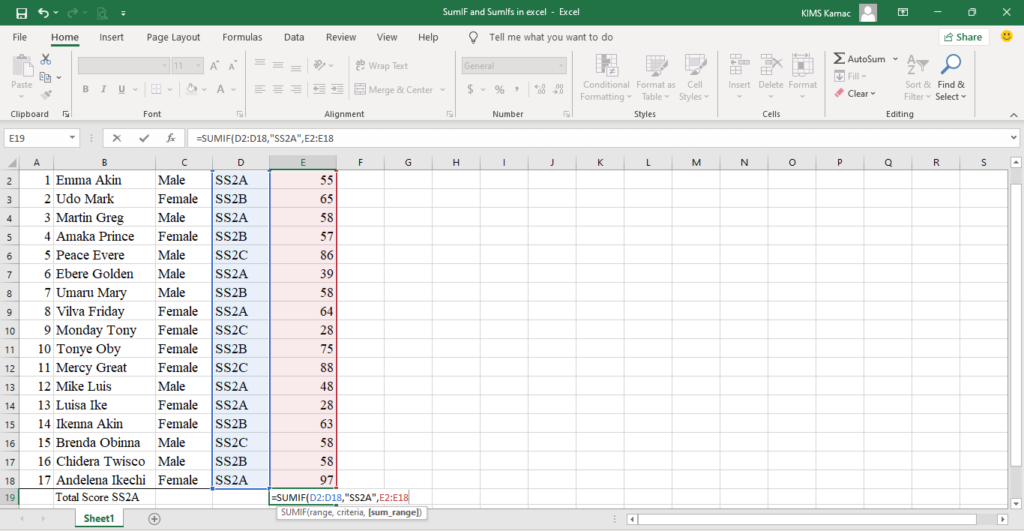
The SUMIF in Excel is used to calculate the total values of a range of cells, based on specified criteria. For example, the worksheet below displays the English score of students based on sex and class. To calculate the total score of students in SS2A, I will use the SUMIF function as follow: =SUMIF(D2:D18, “SS2A”, E2:E18)
The above function states that Microsoft Excel should sum the values in the range E2 to E18 if the value in the range D2 to D18 is SS2A. To execute the function, Excel will trace where SS2A appears in column D and select the corresponding value in column E. When all items are selected, they will be summed together to get the total value.
You can also perform SUMIF in one column only. For example, I can decide to sum the values of those who scored below 50 in English. In this case, it doesn’t matter which class the student belongs to.
To do this, I will execute the following function: =SUMIF(E2:E18,“<50”). In this example, my criteria are less than 50. This leads us to the SUMIF syntax.
The SUMIF syntax
The syntax for the SUMIF function is given by: SUMIF(range, criteria, [sum_range])
Where:
- range: is an argument that must be specified (required). This argument represents the range of cells that should specify the SUMIF criteria. See the example above. Such ranges can contain text, numbers, references, and dates.
- criteria: This is also a required argument that must be specified in the function. The criteria can be a number, text, cell reference, or function. It is used to define the cells that will be summed. When the criteria specified are met, the corresponding cells will be added. Criteria can also accept wild characters such as ? or *. The ? is used to match a single character while * is used to match a sequence of characters. A single character match can be like this, “f?r”. It will match farm, far, Farouk, etc. A sequence character match can be:
- *oon: referring to cells that end with noon. E.g. afternoon, honeymoon, etc
- Good*: referring to cells that begin with good. E.g. good morning, good day, etc,
- *m*: referring to cells that contain ‘m’. e.g. Amaka, Amara, etc.
- sum_range: This is an optional argument in the SUMIF function. This means that this argument may be omitted. However, you can omit it if the sum_range is the same as the range argument. Generally, if this argument is omitted, Excel will always compute the argument based on the range argument. But if the range argument is not a number, an error will occur. It is advised that the sum_range be the same size and shape as the range argument. If their sizes differ, it might affect the performance of the function.
Example of SUMIF function
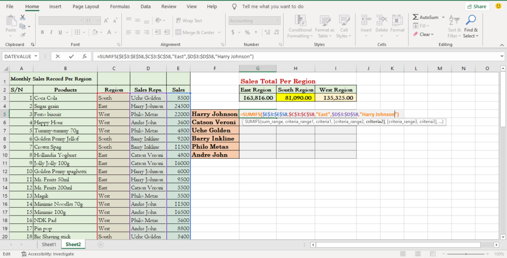
The worksheet below displays the sales record of Wamco Int’l in three regions: East, West, and South. The general manager wants to know the total sales per region for the month under review. You can use the SUMIF function to analyze the data whereby the regions will form the criteria for the sum.

The solution is given as follow:
- Create three columns to represent the total for East, South, and West as illustrated in the worksheet above.
- Under the eastern region cell, enter the formula: =SUMIF($C$3:$C$58,”East”,$D$3:$D$58)
- Copy the above formula and paste it into the remaining two cells.
- Change “east” to “south”, and “east” to “west” respectively.
The SUMIFS in Excel
The SUMIFS in Excel is used to calculate the total values of a range of cells, based on more than one criteria. The SUMIFS function can allow up to 127 range/criteria pairs when analyzing data in Microsoft Excel. Unlike in the SUMIF function where the range to be summed appears last, in the SUMIFS, the sum_range comes first.
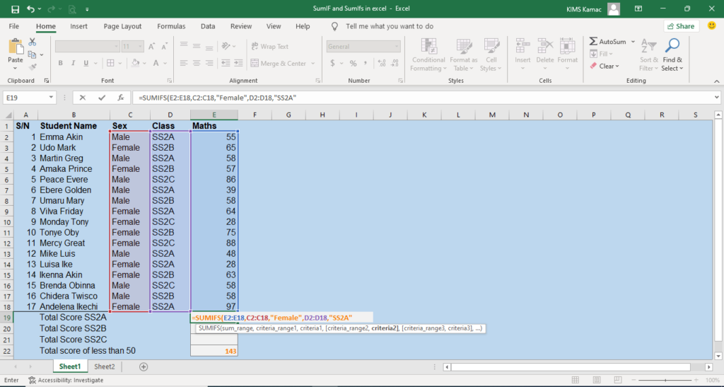
For example, the worksheet below displays the Maths score of students based on sex and class. To calculate the total score of female students in SS2A, I will use the SUMIFS function as follow: =SUMIFS(E2:E18,C2:C18,”Female”,D2:D18,”SS2A”)

The above function states that MS Excel should sum the values in the range E2 to E18. This sum will be calculated if the value in the range C2 to C18 is Female, and the value in D2 to D18 is SS2A. This means that the calculation will be performed only if the Female in columns C matches with SS2A in column D.
To execute the function, Excel will trace where Female appears in column C, and where SS2A appears in column D and select the corresponding value in column E. When all items are selected, they will be summed together to get the total value.
The SUMIFS syntax
The syntax for the SUMIFS function is given by: SUMIFS(sum_range, criteria_range1, criteria1, [criteria_range2, criteria2, … criteria_rangen, criterian])
Where:
- sum_range: is an argument that must be specified (required). This argument represents the range of cells that should be summed. See the example above. Such ranges can contain numbers.
- Criteria_range1: This is also a required argument that must be specified in the function. The criteria_range1 and criteria1 set up a search pair so that the item in criteria1 will be searched for in criteria_range1. If a match is found, the sum takes place, else, the sum is omitted.
- criteria1: criteria1 is a required argument. It defines which cells in criteria_range1 will be summed in the function. The criteria can be a number, text, cell reference, or function. When the criteria specified are met, the corresponding cells will be added. Criteria can accept wild characters such as ? or *. The ? is used to match a single character while * is used to match a sequence of characters. A single character match can be like this, “f?r”. It will match farm, far, Farouk, etc. A sequence character match can be:
- *oon: referring to cells that end with noon. E.g. afternoon, honeymoon, etc
- Good*: referring to cells that begin with good. E.g. good morning, good day, etc,
- *m*: referring to cells that contain ‘m’. e.g. Amaka, Amara, etc.
- criteria_range2, criteria2 … criteria_rangen, criterian: These are optional ranges and criteria up to 127 range/criteria pair. It is used to define the number of range/criteria pairs for the SUMIFS function. Any of them can be omitted in the function. It is advised that the sum_range be the same size and shape as the criteria_range, criteria pair. If their sizes differ, it might affect the performance of the function.
Take note of the following when using the SUMIFS function:
- Always ensure that text values are in quotation marks when specifying criteria. E.g. “Male”.
- Use wild characters to help match multiple cells.
- Ensure that the sum_range contains the same number of columns and rows as the criteria_range argument.
- You can introduce the comparison operators when using the SUMIFS function. For example, =SUMIFS(A2:A10,B2:B10, “>=25”,…)
Example of the SUMIFS function
The worksheet below displays the sales record of Wamco Int’l in three regions: East, West, and South. Each region is controlled by two sales representatives. The general manager wants to know the total sales per sales rep. in each region for the month under review.
You can use the SUMIFS function to analyze the data whereby the sales reps and the regions will form the criteria for the sum.

The solution is given as follow:
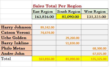
- Create three columns to represent the total for East, South, and West as illustrated in the worksheet above.
- Create six rows to represent each sales rep in each region as shown in the worksheet above.
- Under the east region and the corresponding cell for Harry Johnson, enter the formula: =SUMIFS($E$3:$E$58,$C$3:$C$58,”East”,$D$3:$D$58,”Harry Johnson”)
- Copy the above formula and paste it on the eastern region corresponding to Catson Veroni. Change “Harry Johnson” to “Catson Veroni”.
- Under the south region and the corresponding cell for Uche Golden, enter the formula: =SUMIFS($E$3:$E$58,$C$3:$C$58,”South”,$D$3:$D$58,”Uche Golden”)
- Copy the above formula and paste it on the south region corresponding to Barry Inkline. Change “Uche Golden” to “Barry Inkline”.
- Under the west region and the corresponding cell for Philo Metas, enter the formula: =SUMIFS($E$3:$E$58,$C$3:$C$58,”West”,$D$3:$D$58,”Philo Metas”)
- Copy the above formula and paste it on the west region corresponding to Andre John. Change “Philo Metas” to “Andre John”.
The result shows the total sales each sales representative was able to achieve in the period under review. Harry Johnson made the highest sales while Uche Golden made the least sales.

Conclusion
The SUMIF and SUMIFS in Excel are very useful in data analysis. It helps us to compute totals based on specified criteria. We can use it to compute templates that will run even in our absence.
The SUMIF function requires one criterion while the SUMIFS require multiple criteria. The major difference in their syntax is that:
- In the SUMIF function, the sum_range could be optional and comes as the last argument.
- In the SUMIFS function, the sum_range is required and comes as the first argument.
Haven learned of these functions; you can start implementing them to relevant data. If you encounter difficulties when using them, contact us.
Do not forget to check our previous tutorials in this series:
- What is Microsoft Excel: Tutorial 1
- Entering and formatting data in Excel: Tutorial 2
- Conditional formatting in Excel: Uses and Applications
- Formatting Numbers and Worksheet in Excel
- What is Cell Referencing in Excel?
- Understanding How to Use Excel Formulas and Functions
Next week, we shall discuss the COUNTIF and COUNTIFS functions. Meanwhile, share this with your friends and colleagues.


