The INDEX MATCH function is used to perform a two-way lookup to extract values from a data table. It is used as a substitute to vlookup multiple criteria in Excel before the introduction of the xlookup function.
Remember that the vlookup function cannot perform vertical and horizontal lookup at the same time. To perform a multiple criteria lookup in Excel 2019 and lower versions, we employ the INDEX MATCH MATCH function.
INDEX MATCH function combines two Excel lookup and reference functions category – the INDEX function and the MATCH function. The INDEX function returns a value using a known row and column number. But the MATCH function returns the relative position of a specified item within a range.
When both functions are combined, we can return a value using vertical and horizontal arrays. This helps us to perform a lookup with multiple criteria in Excel without using the VLOOKUP or HLOOKUP functions. In this tutorial, you will learn how to use the INDEX MATCH MATCH formula.
INDEX Function in Excel
The INDEX function is used to return a value within a range in a worksheet. To use the INDEX function, data will be arranged in rows and columns. And each row and column will be numbered from 1 – n.
For example, the table below shows the list of students in a given class. The columns are numbered 1 to 5 and the rows are numbered 1 to 10.
| 1 | 2 | 3 | 4 | 5 | Row/ Column Nos. |
| S/N | Student Name | Sex | Class | First Term | 1 |
| 1 | Emma Akin | Male | SS2A | 92 | 2 |
| 2 | Udo Mark | Female | SS2B | 58 | 3 |
| 3 | Martin Greg | Male | SS2A | 65 | 4 |
| 4 | Amaka Prince | Female | SS2B | 85 | 5 |
| 5 | Peace Evere | Male | SS2C | 57 | 6 |
| 6 | Ebere Golden | Male | SS2A | 69 | 7 |
| 7 | Umaru Mary | Male | SS2B | 68 | 8 |
| 8 | Vilva Friday | Female | SS2A | 86 | 9 |
| 9 | Monday Tony | Female | SS2C | 92 | 10 |
To use the index function to return a value in a range or table, you will specify the array and the row and column numbers.
Syntax of the INDEX function
The INDEX function is given by the following:
=INDEX(array,row_num,[column_num]) – array form =INDEX(reference,row_num,[column_num],[area_num]) – reference form
Where;
- array is required. This is a range of cells from where a value will be returned. If one row is selected, the row_num is optional, similarly, if one column is selected, the col_num is optional.
- reference is required. This is representing a reference to one or more ranges of cells from where a value will be returned. If the references to the ranges are non-adjacent, enclose them in parenthesis, e.g. (A2:B5, A10:B15). If each area in the reference has only one row or column, then the row_num or column_num is optional.
- row_num is required if a column is present. This is the row number in the array or reference from where a value should be returned. It is optional if only one row is selected.
- column_num is required if a row is present. This is the column number in the array or reference from where a value should be returned. It is optional if only one column is selected.
- area_num is optional. This is the area number of the reference from where a value should be returned. According to how the areas are selected, the first area becomes area_num 1, the second area, area_num 2, etc.
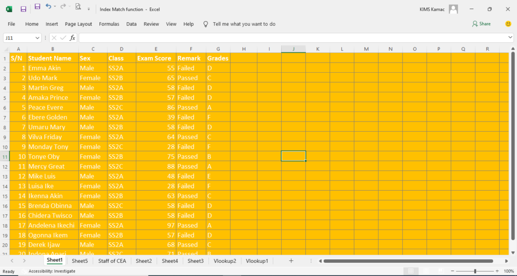
The second INDEX formula is called the reference form. It is usually used when area references are from non-adjacent selections. In this case, we enclose the areas with a parenthesis. Let us use the worksheet below to illustrate.
In the above worksheet, I can include only the following fields: S/N, Student name, Sex, and Exam score, and Remark. This will result in the following areas: A1:C20, and E1:F20. Where A1:C20 is area_num 1, and E1:F20 is area_num 2.
Therefore, to return the student’s exam score in row 7, the formula will be =INDEX(($A$1:$C$20,$E$1:$F$20),7,1,2). Where $A$1:$C$20 is area 1, and $E$1:$F$20 is area 2. The row_num is 7, and the value to return is located in column_num 1 of area_num 2.
Example of the INDEX function
The worksheet below shows the number of students in SS2 offering different courses. Using the index formula,
- How many students in SS2D are offering Mathematics?
- How many students are offering Economics?
Solution
To solve the above problem, let us do the following:
- Create a worksheet with the above data
- Number the columns and rows: there are 12 rows and 6 columns
- Select the cells where the results will appear (see solution below).
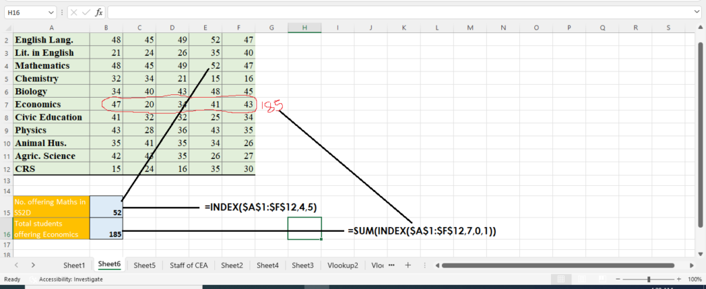
- For No. of students offering Mathematics in SS2D, enter the formula: =INDEX($A$1:$F$12,4,5). Note that: the row_num is 4 and the column_num is 5, using the given array.
- For the total number of students offering Economics, enter the function: =SUM(INDEX($A$1:$F$12,7,0,1)). Note that: we used the reference form where 7 is the row_num, 0 the column_num, and 1 the area_num. We used the sum function to get the total for row 7 which is Mathematics.
The result of the above solution is shown in the image below.
MATCH Function in Excel
The MATCH function is used to return the relative position of a specified item within a range of cells. In this case, the required item is known but the position of the item within a range is not known.
Like in the INDEX function, the MATCH function will automatically number the items in a selected range. It will then return the position number of the item you are searching for. For example, in the table below, the position of Biology is 5, and SS2B is 2, depending on the selected range.
| 1 | 2 | 3 | 4 | 5 | ||
| SS2A | SS2B | SS2C | SS2D | SS2E | ||
| 1 | English Lang. | 48 | 45 | 49 | 52 | 47 |
| 2 | Lit. in English | 21 | 24 | 26 | 35 | 40 |
| 3 | Mathematics | 48 | 45 | 49 | 52 | 47 |
| 4 | Chemistry | 32 | 34 | 21 | 15 | 16 |
| 5 | Biology | 34 | 40 | 43 | 48 | 45 |
| 6 | Economics | 47 | 20 | 34 | 41 | 43 |
| 7 | Civic Education | 41 | 32 | 32 | 25 | 34 |
| 8 | Physics | 43 | 28 | 36 | 43 | 35 |
| 9 | Animal Hus. | 35 | 41 | 35 | 34 | 26 |
| 10 | Agric. Science | 42 | 43 | 35 | 26 | 27 |
| 11 | CRS | 15 | 24 | 16 | 35 | 30 |
Therefore, when you know the item, you are looking for, but want to find its position, use the MATCH function.
Syntax of the MATCH function
The MATCH function is given by the following: =MATCH(lookup_value,lookup_array,[match_type])
Where;
- lookup_value is required. It represents the item or value you want to know its position in the lookup_array. For example, SS2B, in the table above. SS2B is the lookup_value. The lookup_value can be a text, number, or cell reference,
- lookup_array is required. This represents the range of cells from where to search for the lookup_value.
- match_type is optional. This option will tell Excel how to match the lookup_value. There are 3 options:
- 1 – This is the default match_type. It finds the largest value that is less than or equal to the lookup_value. When used, the items in the lookup_array MUST be arranged in ascending order. If match_type is omitted in the MATCH function, this option takes effect.
- 0 – This option is used to search for the exact match of the lookup_value. If there is more than one match, the position of the first value will be returned.
- –1 – This option finds the smallest value that is greater than or equal to the lookup_value. When used, the items in the lookup_array MUST be arranged in descending order.
Example of the MATCH function
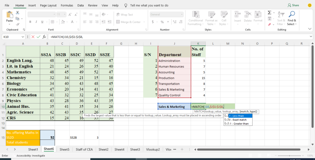
The worksheet below shows the number of staff in ABC Logistics. Use the match formula to locate the position of the Marketing department.
Solution
To solve the above, let us do the following:
- In the worksheet, specify a cell where the result will appear. Let the lookup_value appear at the top or to the left of the output cell.
- On the output cell, enter the formula: =MATCH(J10,$J$1:$J$8,0). Note: Select the lookup_value on the left of the output cell (J10). Then select the lookup_array which is ($J$1:$J$8); finally, specify the exact match which is 0. Press ENTER to display the result.
- The value returned is 7. Remember that this is the relative position counting from the top, not the no. of staff in the dept.
INDEX MATCH Function in Excel
Looking at the INDEX and the MATCH functions, you will observe that they are opposite of each other.
This means that if we don’t know the row_num and the column_num, we can use the MATCH function to get them. This brings us to INDEX MATCH in Excel.
In INDEX MATCH in Excel, we use the MATCH function to provide the row_num or column_num within the INDEX function. To use the INDEX MATCH function in Excel, we rewrite our function as follow:
- =INDEX(array,MATCH(lookup_value,lookup_array,[match_type]),column_num). Here, the row number is unknown but the column number is known.
- =INDEX(array,row_num, MATCH(lookup_value,lookup_array,[match_type])). Here, the column number is not known but the row number is known
- =INDEX(array,MATCH(lookup_value,lookup_array,[match_type]), MATCH(lookup_value,lookup_array,[match_type])). Here, both row and column numbers are not known.
Let us illustrate how to use each of the above formulas with examples.
Index Match with Multiple Criteria:
The INDEX MATCH with multiple criteria is simply using the INDEX and MATCH function for a two-way lookup. To illustrate this, we use two examples where the row number is known and the column number unknown, and vice versa.
Example of Index Match multiple criteria rows and columns
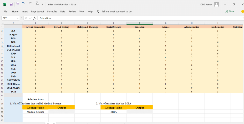
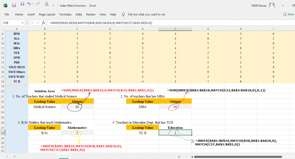
The worksheet below displays the number of staff in a Classical Secondary School, Ipanja. The teachers’ names are arranged based on qualifications.
Use the INDEX MATCH function to solve the following:
- The number of teachers that studied Medical Science.
- The number of teachers that have MBA.
- Find the number of B.SC holders that teach Mathematics
- The number of teachers in the Education Department that have TC II qualifications.
Solution
The solution of the above questions will help us understand how to apply the INDEX MATCH and INDEX MATCH MATCH. Take the following steps.
1. In the worksheet, specify cells where the results will appear. (See the output below).
2. For question No. (1), enter the following formula in the output cell: =SUM(INDEX($B$2:$K$18,0,MATCH(B23,$B$1:$K$1,0)))
- In this example, the MATCH function is used to return the column_num in the INDEX function.
- The SUM function calculates the total No. of teachers.
- The INDEX function is used to select the area that will be calculated.
- The MATCH function nested in the INDEX function is used to select the column that will be calculated. The result is shown in the image below.
3. For question No. (2), enter the following formula: =SUM(INDEX($B$2:$K$18,MATCH(E23,$A$2:$A$18,0),0,1))
- In this example, the MATCH function is used to return the row_num in the INDEX function.
- The SUM function calculates the total No. of teachers.
- The INDEX function is used to select the area that will be calculated.
- The MATCH function nested in the INDEX function is used to select the row that will be calculated. The result is shown in the image below.
4. For question No. (3), enter the following formula: =INDEX($A$1:$K$18,MATCH(B28,$A$1:$A$18,0),MATCH(C27,$A$1:$K$1,0))
- In this example, the INDEX MATCH MATCH function is used to return the row_num and column_num.
- The INDEX function is used to return the number of B.Sc holders that teach mathematics.
- The result is shown in the image below.
5. For question No. (4), enter the following formula: =INDEX($A$1:$K$18,MATCH(B28,$A$1:$A$18,0),MATCH(C27,$A$1:$K$1,0))
- In this example, the INDEX MATCH MATCH function is used to return the row_num and column_num.
- The INDEX function is used to return the number of TC II holders that teach Education in the school.
- The result is shown in the image below.
Index Match Vs Vlookup
The vlookup function cannot be used to perform a lookup for multiple criteria. To overcome this limitation, we can use the INDEX MATCH functions. This is especially useful for those who are using Excel 2019 and lover versions. If you are using Excel 2021 or Microsoft 365, you can leverage the Xlookup function.
Hence, with the Index Match, you can do more than use the vlookup function. Meanwhile, the vlookup is still relevant for a one-way lookup to avoid unnecessary complications. It is, therefore, necessary to understand when to use any of the functions.
Conclusion
The Index Match function is a way of performing a multiple criteria lookup that does not exist in Vlookup. Therefore, it is important to understand when to use the vlookup and Index Match function to return a value.
There are various use cases where you can deploy the Index Match formula in Excel. All you need is to understand how to use it as explained above.
I believe that this tutorial has helped you build a foundation on Index Match vs vlookup functions. Continuous practice will help you improve and become an expert.
We are open to your questions in case you face any challenges working with the functions. We shall look at the pivot table in Excel by next week. Before you go, please, kindly share with a friend. Don’t forget to visit our previous tutorials if you have not done so.


