What is the difference between Vlookup and Xlookup functions? Vlookup and Xlookup functions are used to extract values in a table of data in Excel. Both are used to query a data table and extract items or values in an Excel table or range. The Xlookup function can be seen as a vlookup multiple criteria.
However, vlookup searches for its values from left to right while xlookup searches in a specified column. Also, vlookup cannot be used to extract more than one value, but xlookup can retrieve an array of values.
Just like the vlookup, the xlookup function is one of the functions in the Lookup and Reference functions category. It is used to search, locate and return an item/ value in a table or range of cells. The xlookup function allows you to look for a search term in a specified column. It will then return a result in a corresponding row from another column specified by the user.
For example, if we have the Reg. number of a student, we can search for and retrieve the student’s name. The difference between vlookup and xlookup here is that the lookup_value must not be in the first column. Therefore, the xlookup function searches for what you want in a range or array and returns the required value.
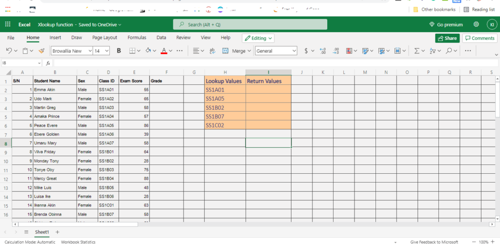
Let us illustrate with this simple example. The worksheet below displays the detail of students in SS1 in a given school. A random sample of 5 students was selected using their Class ID SS1A01, SS1A05, SS1B02, SS1C02, and SS1B07. Use the Xlookup in Excel to return the names of the students.
The xlookup formula in excel is written as follow: =XLOOKUP(Class_ID, the range to look for the value, the range where values will be returned from)
The above explanation will result in the following: =XLOOKUP(H2,$D$2:$D$23,$B$2:$B$23).
Note the following:
- The H2 is the cell reference of the first Class ID. If you copy the formula to the remaining cells, all the results will appear accordingly. You may decide to use each class id instead of cell reference if you are dealing with a few values. In this case, you will have =XLOOKUP(SS1A01,$D$2:$D$23,$B$2:$B$23).
- The absolute range reference, $D$2:$D$23, references the range that contains the value we are searching for. We used absolute reference style so that when we copy the formula, the range will not change. You can also name the range. If you name the range, you will have something like this: =XLOOKUP(F3,Search_range,Return_range).
Where the Search_range is the name of the range to search, and Return_range name of the range to return a value. Naming the range allows you to copy the formula without changing the scope of the data.
- The last 3 entries not included in the function are optional. You can decide to omit them as we did and have the same result. We will talk about them later in the section for the syntax of the xlookup function.
The result of the vlookup formula is given below, check if your result is close to it.
What is Xlookup Function in Excel?
The xlookup function in Excel is one of the recently introduced functions in Microsoft Excel. It is available in Microsoft 365, Microsoft 365 for Mac, Excel for the web, and Excel 2021. It is used to query data to retrieve a value based on available data input.
To use the xlookup formula, we can organize our data in columns and rows. There is no need to put the lookup value towards the left of the return value. The lookup_value column and return value column can assume any position in the data range.
Our example above shows that the lookup value can take any position. As a result, columns are not numbered from the left to the right, as we do in vlookup. Using the xlookup function, we can perform both horizontal and vertical matches as shown in the table below.
| SS1A | SS1B | SS1C | |
| English | 76.5 | 82.1 | 79.6 |
| Mathematics | 78.3 | 65.8 | 71.2 |
| Chemistry | 63.9 | 72.3 | 81.2 |
| Biology | 78.2 | 80.3 | 76.9 |
| Economics | 60.8 | 64.7 | 62.1 |
| Physics | 87.2 | 76.2 | 84.5 |
The table above shows the average examination score of students in SS1 for six subjects. We can use xlookup to retrieve the average score of each class for each subject. To retrieve a value in the above table using the xlookup function, we will use the nested xlookup function.
For example, in the above table, to retrieve the average Biology score, for SS1B, we use the formula: =XLOOKUP(F3,$A$2:$A$7,XLOOKUP(G2,$B$1:$D$1,$B$2:$D$7)). The result will be as follow:
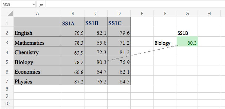
Therefore, we can use the xlookup to perform the functions of vlookup and Hlookup at the same time.
The syntax of the xlookup in excel
The syntax of the xlookup in excel is given by: =XLOOKUP (lookup_value, lookup_array, return_array, [if_not_found], [match_mode], [search_mode])
Where:
- lookup_value is required. It must be specified and represents the value you are searching for, e.g. Class ID. This value can appear in any column in the table. The lookup value can be a number, a text, or a cell reference.
- lookup_array is required also. This represents the range or array to search for the lookup_value. The lookup_array can be a range of cells using absolute cell reference, a named table, or a named range.
- return_array is also required. This is the range or array that contains the value to be retrieved by the xlookup function. As in above, it can be a reference, named table, or range.
- if_not_found is optional. This is used to create a return value if the actual match for the lookup_value is not found. Instead of returning a #N/A error value when lookup_value is not found, use this option. You can specify a return value or a return text in this optional argument. For example, “Class ID not found”. Note: If this option is not specified, xlookup returns #N/A if lookup_value is not found.
- match_mode is optional. By default, xlookup searches for the exact match of the lookup_value. You will use this optional argument to specify the match mode if you do not want the default. There are 4 match modes in xlookup, namely: 0, -1, 1, and 2.
- 0 – This match mode returns the exact match of the lookup_value. If the exact match is not found, it returns #N/A or the value in the if_not_found option.
- -1 – This match mode returns the exact match. If an exact match is not found, it returns the next smaller item.
- 1 – This match mode returns the exact match. If an exact match is not found, it returns the next larger item.
- 2 – This match mode is used to return a wildcard match. ? is used for a single match and * is used for sequence match.
- search_mode is optional. Use this option to indicate how xlookup will search for the required items. There are 4 search modes: 1, -1, 2, and -2.
- 1 – This is the default search mode. It performs a search from the first item on the list.
- -1 – This search mode performs a search in the reverse order. It searches from the last item on the list.
- 2 – This search mode performs a binary search in ascending order. The list must be sorted in ascending order, else, it will return invalid results.
- -2 – This search mode performs a binary search in descending order. The list must be sorted in descending order, else, it will return invalid results.
Vlookup vs Xlookup in Excel
What are the differences and similarities between the Vlookup and Xlookup functions in Excel? The similarities include:
- Both are functions in the Lookup and References category
- Both are used to retrieve values in a range or table of data.
- Both are used to search for items in vertically tabulated data.
- Both search for an item in a specified range and return a value from a specified range.
- Both have the lookup_value as their first argument in their syntax.
Some of the differences between vlookup and xlookup are tabulated below.
| VLOOKUP | XLOOKUP |
| Lookup_value must be in the first column of the table_array | Lookup_value can appear anywhere in the table of data |
| The return value must appear to the right of the lookup column | The return value can appear anywhere in the table of data |
| Searches for items vertically only | Searches for items both vertically and horizontally |
| Cannot be nested in another vlookup function | Can be nested in another xlookup function |
| Uses column index to indicate the column containing the return value | Does not use column index, but return_array to specify column containing the return value |
| Returns #N/A error if the value is not found | Has a parameter to substitute for the #N/A error if the match is not found |
| Returns one item at a time | Returns an array of multiple items |
How to use Xlookup Function in Excel
The xlookup function is an easier function to use than the vlookup function. Because of its simplicity, every excel user should master its usage and use it in place of vlookup and hlookup functions.
We shall illustrate how to use the xlookup in Excel using the following examples. Remember, you should have Excel 2021, Microsoft 365, or Excel for the web to practice these examples.
Example 1: Retrieve multiple items
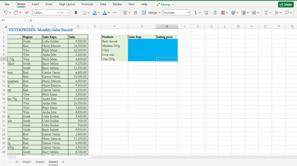
The worksheet represents the sales record of Ugobest Enterprises. Five products were selected from the sales record: Festo biscuit, Minimie 100g, Nibit, Coca cola, and Viva 190g. The management wants to know who sold them and the selling price. Use the xlookup function to retrieve the required values.
Solution
Unlike the vlookup function that retrieves one item at a time, xlookup retrieves an array of multiple items. To solve this problem, we follow these steps.
- Enter the required data in a worksheet or import the data from any source. Note: use Excel for the web if you do not have Excel 2021.
- Create three columns within the worksheet and label them accordingly. See the example above.
- On cell G3, enter the following formula =XLOOKUP(F3,$A$3:$A$52,$C$3:$D$52, “Don’t Exist”). Note: we are using the default match and search mode.
- Copy the formula to the other cells below G3 using the autofill handle.
Notice that both Sales Rep. and Selling price column are populated at once. The result is shown in the table below.
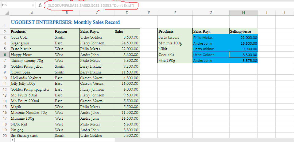
Notice that the function in the sales rep. the column is reflected in the selling price column. You don’t need to replicate them yourself. Note that the wider the scope of your return_array, the more the items to be retrieved.
Example 2: Using match mode
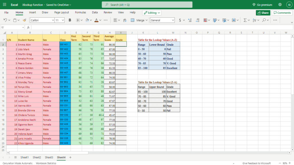
The table below shows the results of students in a given secondary school. The grade obtained by each student is distributed using the following table.
| S/N | Score Range | Grade |
| 1 | 85 – 100 | Excellent |
| 2 | 70 – 85 | V. Good |
| 3 | 60 – 70 | Good |
| 4 | 50 – 60 | Pass |
| 5 | 0 – 50 | Fail |
The average score of each student is shown in the worksheet below. Use the xlookup function to grade each student based on their scores.
Solution
To solve this problem, we’ll first create a table for the lookup value using the range and the grades.
- Create the table for the lookup values and ensure that it is sorted in ascending or descending order as shown above.
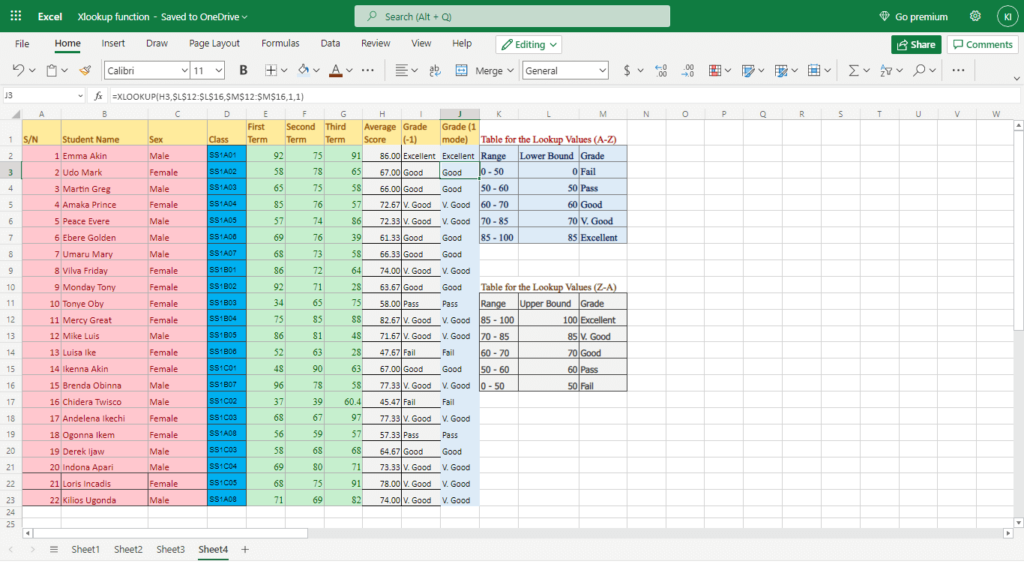
- Under grades, in column I2, enter the following formula: =XLOOKUP(H2,$L$3:$L$7,$M$3:$M$7,”Undefined”,-1,1). This formula is valid for the first table arranged in ascending order (A-Z). The xlookup function will search for and return values equal to or less than the lookup_value from the return_array.
- If you are using the second table arranged in descending order (Z-A), then enter the following formula: =XLOOKUP(H2,$L$12:$L$16,$M$12:$M$16,1,1). The xlookup function will search for and return values equal to or more than the lookup_value from the return_array.
- Copy the formula to other cells using the autofill handle. The results are shown in the figure below.
Example 3: Combining xlookup with other functions
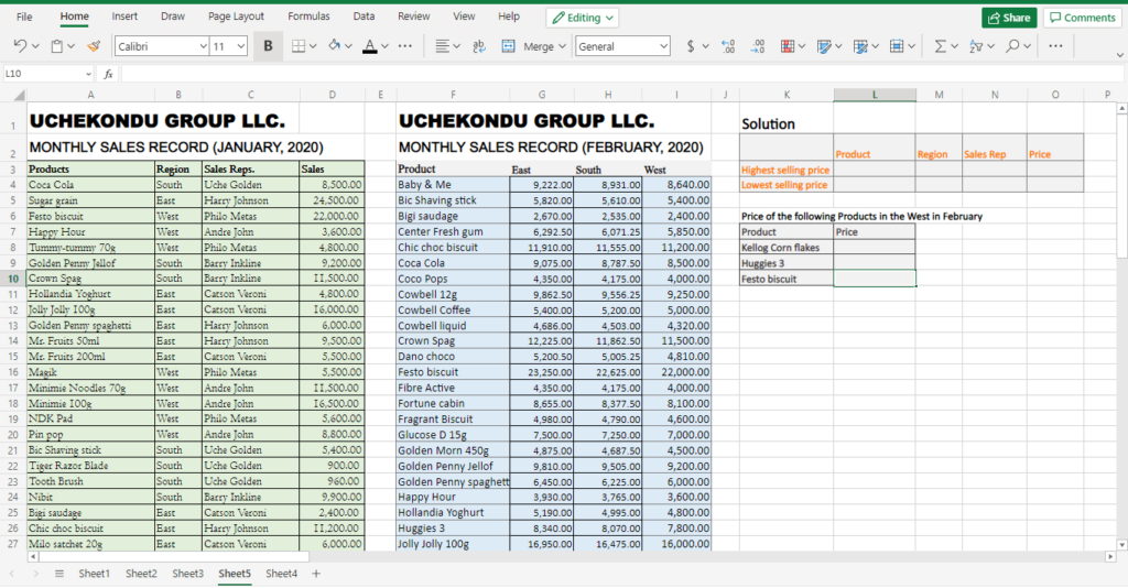
The worksheet below shows the monthly sales record of Uchekondu Group Llc for January and February. Use xlookup to:
- Get the product with the highest selling price, the region, and the sales rep. in January
- The product with the lowest selling price, the region, and the sales rep. in February
- The price of Kellog Corn flakes, Huggies 3, and Festo biscuit in the West in February.
Solution
The Solution to the above problems is straightforward. Only that we will include another function in the xlookup function. Firstly, create columns where the results of the search will appear, as shown in the worksheet above.
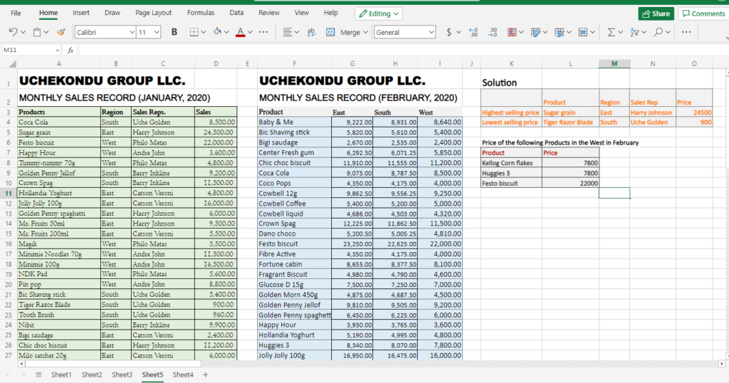
- On cell L3 under product, enter the following formula: =XLOOKUP(MAX($D$4:$D$53),$D$4:$D$53,$A$4:$D$53,”Wrong”,1,1). We used the MAX function to locate the maximum (highest) selling price. So our lookup_value is the maximum value. We then return the product, region, sales rep, and price associated with the highest selling price.
- Copy the formula above and paste it in cell L4, and change the MAX function to MIN. the formula is: =XLOOKUP(MIN($D$4:$D$53),$D$4:$D$53,$A$4:$D$53,”Wrong”,1,1). The MIN function locates the lowest selling price. Then the rest of the function returns items associated with the lowest selling price.
- In the third question, use the nested xlookup to get the intersection of the products and the West region. Enter the following formula in cell L8: =XLOOKUP(K8,$F$4:$F$59,XLOOKUP(“West”,$G$3:$I$3,$G$4:$I$59, “Error”)). Use the autofill handle to copy the formula downwards.
The result of the above solutions is given in the worksheet below. To download the workbook for the above examples, click here.
Conclusion
The xlookup function is easier to use than the vlookup function. It is also more useful since it can return an array of multiple items.
The xlookup function has a parameter that can be used to return a specified option if an error occurs. There are various use cases where you can deploy the xlookup formula in Excel. All you need is to understand how to use it.
I believe that this tutorial has helped you build foundational knowledge on how to use the xlookup formula in Excel. If you keep practicing, you will understand it more. We are open to your questions in case you face any challenges while your newfound function. We shall look at the INDEX MATCH functions by next week. Before you go, please, kindly share with a friend. Don’t forget to visit our previous tutorials if you have not done so.


